Introduction
Before we start reading the chapter, I’d like to give you a brief introduction to the two main ideas.
Note that this chapter heavily uses the material of Preamble Assignments #2, 3, and 4. Hopefully you have had a chance to work through these by now. If you haven’t had a chance to work through these yet, go ahead and start reading the notes below, but when you see something unfamiliar, refer back to those assignments for more background.
The Binomial Distribution
The first idea has to do with one of our questions in the introductory lecture: if we flip a coin 10 times, which is more likely, HHHHHHHHHH, or HHTTHTHHHT?
The answer you have found, by now, is that they are both equally likely: each has probability $(1/2)^{10}=1/1024$, about 0.1% chance each. Every sequence of ten H’s and T’s has equal probability.
One reason the first sequence looks less likely is because it looks “special”. Of course, every sequence is equally “special”.
A little more specifically, when we are looking at the second sequence, I think that perhaps we are unconsciously thinking “what is the probability of a sequence like this one?”, not “what is the probability of this sequence exactly?”. Which is a very different question.
What do we mean “a sequence like this one”? There are many possible answers. The simplest and crudest answer is just counting the H’s and T’s. So we might be unconsciously asking, “what is the probability of 10 H’s?”, versus “what is the probability of 6 H’s?”. And those questions do have different answers!
The number of ways of getting 10 H’s is only $(1/2)^{10}$, because there is only one way to do it. But, recalling Preamble Assignment #2, the number of distinct sequences with 6 H’s is $$\binom{10}{6}=210,$$ because there are 6 choices of which places in the sequence are H’s.
(Let me briefly remind you how that goes. We choose 6 of the 10 places in the sequence to be Heads. Choosing one place, there 10 choices, then 9 choices for the next place, then 8, down to 5 choices for the last place, so $10\times 9\times 8\times 7\times 6\times 5$ choices overall. But if I had chosen the places for the heads in a different order, it would not have mattered! So I have over-counted by a factor of all the different orders I could have chosen those same six places: $6\times 5\times 4\times 3\times 2\times 1$. To get the number of ways the six Heads could be distributed in the ten places, I need to divide my initial count by my over-counting factor. The symbol for this number is $\binom{10}{6}$, read “ten choose six” (number of ways to pick six things out of 10), and it works out to $$\binom{10}{6}=\frac{10\times 9\times 8\times 7\times 6\times 5}{6\times 5\times 4\times 3\times 2\times 1}=210.$$ See Preamble Assignment #2 for more detail.)
This in turn means that the probability of getting 6 H’s is $\binom{10}{6}(1/2)^{10}=210(1/2)^{10}\doteq 0.205$. The probability of 10 H’s is less than 0.1%, but the probability of 6 H’s is about 20.5%, or 210 times greater.
This is one way of expressing our intuition that HHHHHHHHHH is “more special” than HHTTHTHHHT. Note that it does NOT change the fact that these two PARTICULAR sequences are equally likely.
In a similar way, we could calculate the probability of getting $k$ heads in $n$ flips of the coin. If our sample spaces points are “the number of heads obtained” (so $S=\{0,1,2,\dotsc,n\}$), then assignment of probabilities to those points is called the Binomial distribution (because the formula uses the binomial coefficient).
More generally, the probabilities of H and T don’t have to be 0.50 each; we could for example roll a die repeatedly, and ask how many 1’s we get. We can find the probability by the same process.
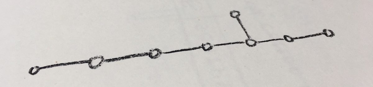
One way to picture the binomial distribution for a coin—and to connect it to Pascal’s triangle—is to imagine a ball being dropped into a triangular maze. At each level of the maze, it can go either left or right.
If the maze is 10 levels deep, then each path through the maze corresponds to a sequence of L’s and R’s 10 letters long. All the sequences with 6 L’s end up in the same final location.
Exercise 1:
a) Convince yourself of what I said above!
b) Verify that the numbers of Pascal’s Triangle count the number of paths through the maze in exactly this way. (Just do the explicit counting for the first few levels of the maze/triangle. If you are feeling ambitious, you could try to write a proper proof, but only do that if you feel the need to practice proof writing…)
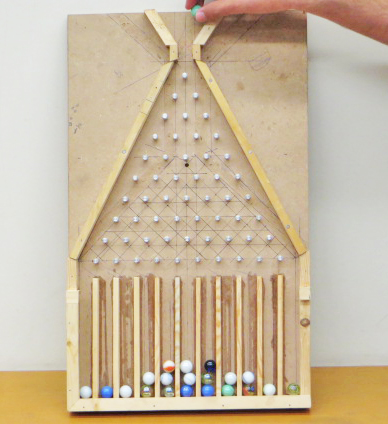
If all the L’s and R’s are equally likely, we will end up with more marbles towards the center, because there are more different paths to the spots near the center than there are towards the edges.
This maze is sometimes called a “Galton board”, or a “triangular Plinko game”. See this page from PhysLab for pictures of a physical board, and this page (from Bob Lochel) for some videos and simulations.
The poisson distribution
This goes back to our question in the introduction, about the lottery: if we play a lottery with a p=1/1,000,000 chance of winning each time, and we play it n=1,000,000 times, what is our chance of winning at least once?
Let W be the event that we win at least once. Then W’ is the event that we win 0 times. But P(W’) is easier to calculate than P(W). If we imagine winning as Tails, then we are asking for the probability of a sequence of 1,000,000 Heads (or losses). The probability of loss is q=(1-p), so $$P(W’)=(1-p)^n.$$ Now, in our particular example, we had p=1/n, so $$P(W’)=\left(1-\frac{1}{n}\right)^n.$$
This should look familiar from both Preamble Assignment #2 and #3!
We could also ask: if we play a lottery with a p=1/1,000,000 chance of winning each time, and we play it n=1,000,000 times, what is our chance of winning exactly once? We could approach this question in a similar way. Or we could ask, what is our chance of winning exactly twice?
Continuing this line of reasoning leads to the Poisson distribution. I’ll wait until we get to it in the book to say more.
(Note that the Poisson distribution will not be of interest only for winning lotteries; we can also use this distribution in any case where there is a certain probability of an event happening per unit time, and we want to know what is the probability of a certain number of events in a given time period. An important example is nuclear decay.)
THE READING
OK, let’s start reading the text. I will again give less detailed notes than I did for the first two chapters. Keep up with the usual techniques:
- Read slowly
- Keep notes
- Invent examples
- Verify all statements yourself
- Make summaries
1. Bernoulli Trials
(Pages 146–147)
Everything in this section is important. Hopefully this is not too hard. Don’t worry about calculating the probability of a “royal flush” (or even what that is). The conceptual points he makes, about whether a coin has a memory, and about whether certain other processes are well-modeled by Bernoulli trials, are important.
Exercise 2: Come up with some examples that (a) would, and (b) would NOT, be well-modeled as Bernoulli trials.
2. The Binomial Distribution
(Pages 147–150)
The most important sections in this chapter are 2, 5, and 6. Section 2 is about 50% of the most important topics. Most of the material in this section is very important, except for some details of some of the examples. Don’t worry if you need to spend a good amount of time on this section; several of the later sections we will skip over quickly.
Make sure you thoroughly follow the derivation of the Theorem near the top of page 148.
Don’t worry if the term “random variable” seems vague: we will return to this in a much detail in the next chapter.
Exercise 3: In the third paragraph of page 148, the author makes the claim that “(2.1) represents the kth term of the binomial expansion of $(q+p)^n$”. Make sure you fully understand why this is true! Also make sure you understand why this implies $(q+p)^n=1$, as the author states in the next line.
This is all pretty theoretical. It will be helpful to see numerically and graphically what is going on:
Exercise 4:
a) Suppose we are flipping a coin 10 times. Use a Pascal’s triangle to calculate numerically the probability of 0, 1, 2, … , 10 heads, entering the numbers in a table. Graph these numbers, using a bar graph. (I STRONGLY recommend doing the Pascal’s triangle and the graph by hand—I think it is very instructive to see explicitly how the numbers work out and how the graph looks. You can use a calculator for the probabilities, but at this level of accuracy you should find that you can do them by hand as well. You don’t have to be super-accurate with the graph, but don’t be super-messy either.)
b) Suppose that we are rolling a die 10 times. “Success” is rolling a five or a six. Repeat part (a) in this case, finding the probability of 0, 1, 2, … , 10 successes, and so on. Re-use your work where possible. Use a calculator where needed.
c) Suppose that we are doing something with a probability p=1/10 of success, and we are repeating it 10 times. Repeat (a) and (b) in this case. Do you see how and why the binomial distribution gets shifted over?
Continuing reading: Example (a) is worth following. Probably it is clear how to compute the theoretical values in Table 1; you might try a couple to be sure. You can skip Example (b), because it refers to combinatorics from Chapters IV and II which we skipped. You should verify the calculation of Example (c); it uses a logarithm, see Preamble Assignment #3 if you are rusty on those.
Example (d) is an example of a situation where it isn’t obvious at first that a binomial distribution could be applied. You should be able to check the author’s numbers, but the more important thing is to check that you understand how the binomial distribution is being applied.
Similarly, the way the binomial distribution is applied in Examples (e) and (f) is kind of tricky. (Note that “serum” is an old word for “vaccine”: the “serum” is supposed to prevent the disease.) It took me a few runs through reading this example to keep the reasoning straight in my mind. I would recommend doing that, checking the author’s numbers, and maybe making up other numbers of your own. The reasoning here is more important than the particular numbers.
3. The Central Term and the Tails
I am going to break from my usual rule here, and try to explain this section to you, rather than have you work through it. The author is trying to be more theoretical here than I want to be. I will explain what I think are the main important points. I think it will be helpful then to look at what the book says, to avoid being intimidated, but you don’t have to work through everything in detail. (If you want to, you can take working through this section as a challenge exercise!)
Here are my main points I take from this section:
1. The binomial distribution is “bell-shaped”. If we graph it, with the number of successes on the x-axis, then moving left to right (increasing number of successes), it starts off small, increases slowly at first and then rapidly to a maximum, then decreases in a similar way.
2. The maximum point of the binomial distribution—the most likely number of successes—occurs at or near np, where n is the number of trials, and p is the probability of success.
3. The “tails” of the distribution are quite flat: it is quite unlikely that the number of successes deviates very “far” (in some appropriate sense) from equaling np.
Here are some pictures. I calculated them using an app created by Matt Bognar of University of Iowa. You can find it here ; I recommend playing around with it a bit.
Here’s what it looks like for 10 coin flips, “success” being a head (n=10, p=0.5):
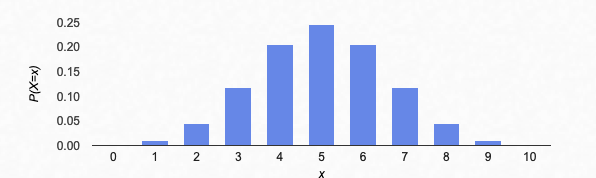
Is it clear how to read the graph above? For example, do you see that the probability of getting exactly 7 heads in 10 coin flips is somewhere between 0.10 and 0.15 (10 and 15 percent)?
Here’s what it looks like for 100 coin flips, “success” again being a head (n=100, p=0.5):
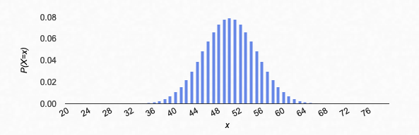
You see what I mean by a “bell” shape? The most likely number of heads in 100 flips is 50, so that is the maximum of the distribution. Roughly speaking, the most likely number of heads in n flips is (1/2)n = np. (This isn’t exactly correct because np might not be a whole number; I’ll return to this below.)
You can see also that the tails are pretty flat: from the graph, it looks like there is almost no chance of getting fewer than 30 or more than 70 heads. (We’ll make this more precise as we go on.)
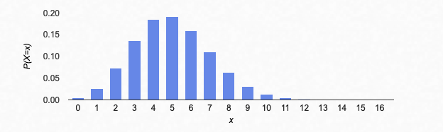
For coins, the distribution is symmetric. That won’t be true if p is not 0.5. For example, let’s see what it looks like for dice rolls: let’s roll a die 6 times, and let a “success” be rolling a six. How many sixes should we expect? Here’s the binomial distribution for that problem, with n=6 and p=1/6:

Getting 1 six is the most likely outcome, but getting no sixes or 2 sixes are also pretty likely. The probability drops off rapidly to get 3 or more sixes (though it’s still definitely possible).
Let’s try it again, with 120 rolls of the die, and success being rolling a six (n=120, p=1/6):
In 30 rolls, what’s the most likely number of sixes? It’s 30(1/6)=5. In general, with n rolls of the die, the most likely number of sixes is (1/6)n. If the probability of success was p, the most likely number of successes is np.
There’s one more point to make: although np is the most likely number of successes, it’s not actually that likely if n is large. For example, if we flip a coin 100 times, it’s not all that likely that we get exactly 50 heads (the probability is a little under 8%). But that’s where the peak probability is centered.
In Section 3, the author states these properties. He gives a theorem saying my points 1 and 2 above (and making 2 more precise). He gives a formula estimating how small the tails are. Getting such an estimate is often very important. However, the estimate he gives here is not very good; he derives a much better one in the next chapter. So I think it is OK to skip it.
At this point, I’d recommend skimming over the chapter to verify for yourself that the author is saying what I’ve said. You can stop now and jump to the next section.
IF you are interested in reading the section more carefully, here are a few notes. You should take the rest of what I write for Section 3 as strictly optional.
I’d start by reading the Theorem near the top of page 131. That says what I said above. It is more precise about where the maximum of the distribution is. It happens at the number he calls “m“; to see what m is, look at the sentence before the theorem, and formula (3.2). To understand what (3.2) is saying, try it for some examples: I used coin flips, with either n=100 or n=101.
Having read the theorem, if you are interested, you could start again at the beginning of Section 3, where the author gives a proof. (He looks at the ratio of one probability to the next one, and says that this is bigger than 1 (increasing) at first, then switches to less than 1 (decreasing) after some point.)
Starting with the second paragraph after the theorem, the author is making an estimate about how large the tails are, that is, how likely large deviations from np successes are. It will be easier to read this part if you make up some numbers. It will aslo I used n=100 coin flips, success is a head, p=0.5, and I looked for the chance of getting 80 or more heads, $P(S_{100}\geq 80)$. When I used his estimate (3.5), I got that this probability is less than 2%. That is not a very good estimate. We will see in the next chapter that the probability is slightly less than $10^{-9}$. The chance of getting 80 or more heads in 100 coin flips is less than one in a billion.
(Why does the author do a poor estimate, when he does a better one the next chapter? I think he is trying to show what sort of estimate you can get just by simple ideas: looking at that ratio again, and comparing the sum of probabilities for 80 , 81, 82, … ,100 heads to a geometric series. He’s showing how good an estimate you can make now, without introducing more new ideas. The better estimate he gives in the next chapter uses much fancier methods.)
4. The Law of Large Numbers
Again, like with Section 3, I’m going to deviate from my usual rule, and just try to explain this section. The author is trying to be more theoretical here than I am planning to be in this class. However, the key idea in this section is important, and you are likely to meet it if you are applying probability methods in the future.
The question this section talks about is this: suppose I flip a coin n times, and let S_n be the number of heads that come up (“successes”). Then I would expect that the ratio S_n/n should be quite close to 1/2. If I flip a coin 100 times, I would expect the number of heads to be close to 50. Moreover, the ratio S_n/n should be more likely to be close to 1/2, the larger the number n of flips I do. The number of heads should “average out” to 50%, as I do more and more coin flips.
I need to be careful to state this correctly, though. As we say, if I flip a coin 100 times, it’s not that likely that I get exactly 50 heads. And that only gets worse: in 1000 coin flips, getting 500 heads is even more unlikely.
What I want to say is that the ratio S_n/n is getting closer and closer to 1/2, as n gets larger and larger. If you know calculus at all, you are very familiar with statements like this. But in our context of probability, this statement still isn’t quite right: there is still a chance that S_n/n is quite far from 1/2! Maybe we get unlikely in a particular run of n coin flips and get 60% heads (or even 100% heads)! It’s not at all likely, but it could happen. So we need to put that in the statement.
Let’s try again. First, since we don’t expect S_n/n to be exactly 1/2, let’s fix a range around 1/2. To be concrete, let’s say: is it going to be true that $$0.45<\frac{S_n}{n}<0.55\quad ?$$Well, maybe, maybe not. It’s actually not that probable if the n is small (e.g. if we only did n=4 coin flips, it’s only 25% likely that S_4/4 is in that range). But it should get more and more probable as we do more and more coin flips: as n gets larger, $$P(0.45<\frac{S_n}{n}<0.55) \quad\text{approaches}\quad 1.$$Let me make this look more like the book’s statement, (4.1). First of all, there is an algebraic trick which is convenient: we can write the double inequality $0.45<\frac{S_n}{n}<0.55$ as one inequality with an absolute value. I can rewrite $\frac{S_n}{n}<0.55$ as $\frac{S_n}{n}<0.50+0.05$, or equivalently $\frac{S_n}{n}-0.50<0.05$. Similarly, $0.45<\frac{S_n}{n}$ can be rewritten $0.50-0.05<\frac{S_n}{n}$, or $-0.05<\frac{S_n}{n}-0.50$. Both of these together are saying that $\frac{S_n}{n}$ stays within a range of 0.05 of 0.50. But we can write the distance, or range, as an absolute value: both those inequalities can be written as the one statement $$\left\vert\frac{S_n}{n}-\frac{1}{2}\right\vert<0.05.$$It is also standard to write an arrow “$\rightarrow$” for “gets closer and closer to” (or “approaches”, or “limits to”).
So my assertion above can be stated, as n increases, $$P\left(\left\vert\frac{S_n}{n}-\frac{1}{2}\right\vert<0.05\right)\rightarrow 1.$$ This looks more like (4.1)!
Now, I chose the range from 0.45 to 0.55 kind of arbitrarily. The same statement will be true if I replaced 0.05 with 0.01, or even with 0.001. No matter how small I make the range around 0.50, the probability of S_n/n being in that range around 0.50 will approach 100%, as I do more and more coin flips. So rather than 0.05, or 0.01, or 0.001, we replace the 0.05 with $\epsilon$, and say that, for any $\epsilon>0$, as n increases, $$P\left(\left\vert\frac{S_n}{n}-\frac{1}{2}\right\vert<\epsilon\right)\rightarrow 1.$$(The symbol $\epsilon$ is a Greek letter “epsilon”, which is a Greek “e”; I believe it stands for “error”, as in, this is the error of the observed probability of heads versus the true probability. It is a standard letter in math for a small number, usually some sort of “error”.)
Only one other thing to generalize: it didn’t have to be coin flips. If we were doing die rolls or something else, we would have some probability p of success, and we would expect that the ratio of S_n/n should be close to p (instead of being close to 1/2 as it is for coins). Therefore, our final statement is:
Suppose we are looking at a binomial distribution, with n trials and a probability p of success. Then, for any $\epsilon>0$, as n increases, $$P\left(\left\vert\frac{S_n}{n}-p\right\vert<\epsilon\right)\rightarrow 1.$$
You might want to skim through Section 4 now, if you haven’t already. Reading it carefully is strictly optional.
5. The Poisson Approximation
OK, in this section, I’ll return to having you read the book. This section IS important. The most important sections in this chapter overall are Sections 2, 5, and 6. This section, together with 6, is about 50% of the most important material of the chapter.
Before we start reading, let me give you an introduction.
The subject of this section (the Poisson approximation) refers to a situation like Puzzle 1 in the introductory lecture. Recall that puzzle: we have a lottery with a chance $p=1/1,000,000=1/10^6$ of winning each time, and we play it $n=1,000,000=10^6$ times. What is the chance of winning at least once?
The easiest way to approach this problem is to find the probability that we win zero times. The probability of NOT winning each time is $$\left(1-p\right)=\left(1-\frac{1}{10^6}\right).$$ I am assuming that each time we play the lottery is independent, so the probability of losing $n=10^6$ times is $$\left(1-p\right)^n=\left(1-\frac{1}{10^6}\right)^{\left(10^6\right)}.$$Now, you can work this out on a calculator, and it comes out to about 0.3679. So there is approximately a 36.8% chance of winning zero times, and therefore a probability of about 0.6321, or approximately a 63.2% chance, of winning at least once.
We can go further here. First, you may check that we would get the same answers if we played a lottery with a chance of winning $p=1/100$, and we played it $n=100$ times. Or if we played a lottery with a chance of winning $p=1/1,000$, and we played it $n=1,000$ times. What is important is that in each case. the expected average number of winnings $np$ is equal to 1, the probability $p$ of winning is small, and the number of trials $n$ is large.
Secondly, we can come up with an expression for this number. InPreamble Assignment #3, you saw that $$\lim_{n\to\infty}\left(1+\frac{1}{n}\right)^n=e,$$ where $$e\doteq 2.71828182846$$ is the base of natural logarithms. That means, for large $n$, we have $$\left(1+\frac{1}{n}\right)^n\approx e.$$Now, note that in the examples above, $p=1/n$. So the probability of winning the lottery 0 times is $$\left(1-\frac{1}{n}\right)^n$$ for a large value of $n$. Pretty close! Here’s a sneaky bit of algebra to make it closer: define a new variable $m=-n$, so that $(-1/n)=(1/m)$. When $n$ is large, so is $m$. Then, for large $n$, the chance of winning is about $$\left(1-\frac{1}{n}\right)^n=\left(1+\frac{1}{m}\right)^{-m}=\left(\left(1+\frac{1}{m}\right)^m\right)^{-1}\approx e^{-1}.$$ So that number 0.3679 is actually $e^{-1}$ or $1/e$ (check this on a calculator!), and the probability of winning at least once is $$1-\frac{1}{e}\doteq 0.6321.$$
(Side note: I have done something somewhat illegal changing $m=-n$, because I only know that $\left(1+\frac{1}{m}\right)^m\approx e$ for large positive $m$; I don’t know that it works for negative $m$ (it does). It’s not hard to justify this more carefully, but I don’t want to get too far off track. Ask me if you’re interested!)
Alright, we can generalize this reasoning.
EXAMPLE: Let’s say we are again playing a lottery with probability $p=1/1,000,000=1/10^6$ of winning. But let’s say we play it $n=2,000,000=2\times 10^6$ times. What is the probability that we win at least once?
The probability of winning 0 times is $(1-p)^n$, as before. But now $p$ is not $1/n$; actually, with the numbers I gave, $p=2/n$. So the probability of winning 0 times is $$\left(1-\frac{2}{n}\right)^n.$$ Introduce a new variable $m=-n/2$, so that $(-2/n)=(1/m)$, and $n=-2m$. Then $$\left(1-\frac{2}{n}\right)^n=\left(1+\frac{1}{m}\right)^{-2m}=\left(\left(1+\frac{1}{m}\right)^m\right)^{-2}\approx e^{-2}\doteq 0.1353.$$So there is a $1/e^2\doteq 0.1353$ probability of winning 0 times, and hence about a 86.5% chance of winning at least once.
The important thing in this example was how $n$ and $p$ were related. The probability $p$ was small, the number of trials $n$ was large, but the expected number of winnings on average was $np$, which was equal to 2 in this example. Anything with $p$ small, $n$ large, and $np=2$ would have worked out the same way.
Exercise 5:
(a) Suppose that we are again playing a lottery with chance of winning $p=1/10^6$. We play the lottery $n$ times. In the same way as above, calculate the probability of winning 0 times in terms of $e$, if (i) $n=3,000,000=3\times 10^6$, (ii) $n=500,000=0.5\times 10^6$, (iii) $n=\lambda\times 10^6$, where $\lambda$ is a constant.
(b) Suppose that we are playing a lottery with a small chance of winning $p$, and we play it $n$ times. Suppose that the expected average number of winnings $np$ is some constant $\lambda=np$. Find the probability of winning 0 times, expressed in terms of $e$ and $\lambda$. (Hint: write $p$ in terms of $n$ and $\lambda$.)
Note that this problem is a special case of the binomial distribution: we are doing an experiment with probability $p$ of success, and repeating it over $n$ trials. The chance of 0 successes is what the book calls $b(0;n,p)$. The expression you have just worked out is one case of the Poisson approximation to the binomial distribution.
Now let’s look at the book. We are in Section 5, page 153. The beginning paragraphs, including formulas (5.1) and (5.2), are what we just worked out. Jump ahead to (5.4): that should be what you just figured out in Exercise 7. (Go back if it’s not!!)
In (5.3) and the sentence before, the author is working out the formula (5.4) in a different way than we did. You can skip this if you want. But if you are interested, you should be able to follow the author’s derivation here.
Now, what the author is going to next is the following: what is the probability that we win the lottery exactly once? That would be the binomial probability $b(1;n,p)$. It’s possible to start again from the beginning and work this out the way we did $b(0;n,p)$. But the author shows a clever way of piggybacking off the work we have already done.
Exercise 6: This exercise aims to understand formula (5.5). When I am given a formula like this for general $k$, I start with some specific $k$ to see what it says.
(a) Normally I’d start with $k=0$. Do you see why I can’t do that for (5.5)?
(b) Let’s start then with $k=1$. Write out the whole of (5.5) in this case. Now try to prove it: substitute in the formula for $b(k;n,p)$, and try to simplify. Do you get what the author does in the simplification in the first step?
(c) Still with $k=1$: can you see why the approximation in the second step of (5.5) is valid? Remember that $p$ is assumed to be very small; what do you know about $q$?
(d) Now, do the same for $k=2$. Write out the whole of (5.5); substitute in the formulas for $b(k;n,p)$ and simplify; and try to understand the approximation in the last step.
(e) (Optional) Derive (5.5) for any positive integer value of $k$.
Exercise 7:
(a) Prove the approximation for $b(1;n,p)$ that the author gives near the bottom of page 153.
(b) Do the same for the approximation for $b(2;n,p)$ at the bottom of the page.
(c) Work out the approximation for $b(3;n,p)$ the same way.
(d) Can you see how you end up with the approximation for $b(k;n,p)$ given in (5.6)? (You don’t have to prove it with induction, just try to understand how you would get this answer if you continued with $k=4,5,6$, etc.)
Let’s go on to the Examples, starting on page 154.
Example (a) Since this refers to Chapter IV, which we skipped, we might as well skip this example.
Example (b) Note that by “digit”, the author means one of the ten symbols 0, 1, 2,…, 9. I don’t know why he picks this particular example of a random process. You should convince yourself of his assertion that the number of occurrences of (7,7) should follow a binomial distribution with n=100, p=0.01. Don’t worry about the “$\chi^2$-criterion” (Greek letter “chi”, pronounced “kai”); it’s a side note, we might get to this if we have time.
Examples (c) and (d) These are good, typical numerical examples, and you should make sure you understand them. You might want to spot-check his numbers to be sure you are calculating things correctly.
In particular, I find (d) a helpful example, as a typical application of the Poisson approximation. It says, if we are making items in batches and some are defective, if defective items are rare, and the expected number of defective items in a batch is $\lambda$, then the probability of exactly $k$ defective items is given by the Poisson formula (5.7).
Examples (e) and (f) These examples aren’t numerical, but are just different practical examples of situations to which the Poisson approximation would apply. They are worth thinking about a bit.
Exercise 8: Let’s make up a couple of numerical examples, based on the author’s examples, to try to make things concrete.
(a) Suppose that a book has misprints on average about once every ten pages, so that the average expected number of misprints per page is $\lambda=1/10=0.1$. Assume (as the author says in the book) that placing each letter is a Bernoulli trial, with a fixed small probability $p$ of misprint, and that there are a large number $n$ of characters per page, such that $np=\lambda=1/10$. Then find the probabilities of 0, 1, 2, 3, and 4 misprints on a single page. Graph these probabilities as a bar graph (with # of misprints on the x-axis, and probability on the y-axis).
(b) Suppose that muffins have an average number $\lambda=5$ of chocolate chips (who likes raisins??). Assuming the author’s reasoning that the Poisson approximation applies to this situation (he’ll say more in the next section), find the probabilities of 0,1,2,3,4,5,6,7,8,9,10,11,12,13,14,15 chocolate chips. Put your answers in a table, and make a graph.
6. The Poisson Distribution
In this section, the author explains that the Poisson approximation to the binomial distribution, (5.7), can be useful in its own right. In this case, it is called the Poisson distribution. Before we start reading, let me say a couple of things.
The Poisson distribution applies whenever we have a known average number $\lambda$ of events per unit time, with the events distributed randomly in times. For example, we might have a radioactive substance, which produces a known number of decays per minute. Suppose then we want to know, in a given minute, what is the probability of $k$ decays? The most likely number of decays is $k=\lambda$, but it certainly won’t always be exactly $\lambda$; the Poisson distribution (5.7) tells you the probability of $k$ decays in a minute, knowing the expected average number $\lambda$ of decays per minute.
You could also generalize this probability to time periods other than one minute; if the time period is $t$, the probability of $k$ decays in $t$ minutes is given by (6.2).
This equally well works if the events are randomly occurring in space rather than time. If the sky has $\lambda$ observable stars per unit area on average (for some definition of “observable”), then the probability of seeing $k$ stars in any unit of area is given by (5.7), and the probability of seeing $k$ stars in $t$ units of area is given by (6.2).
Alright, let’s start reading.
Page 157, first paragraph: What the author is saying here is that, if we add up the probabilities $p(k;\lambda)$ for all possible values of $k$, that is, $k=0,1,2,3,\dotsc$, then we will come up with probability 1 for any possible outcome, as we must.
Exercise 9: Write out the algebra to prove the statement I just said (which the author explains verbally in this paragraph). You will need the infinite series for $e^x$ that we worked out in Preamble Assignment #4.
Rest of page 157: The author’s main point in this section is in the last paragraph of page 157 (continuing to the top of page 158). If we have a process where events happen randomly in continuous time, with an average number $\lambda$ of events in a time interval, then we can approximate that by dividing time into many small discrete intervals. Then we can think of each discrete interval as a Bernoulli trial, with a small chance of success, and apply the Poisson approximation. This shows that the Poisson approximation applies to random processes with a certain number of “successes” per unit continuous time, like the radioactive decay example I mentioned at the start.
Exercise 10: Write out the author’s argument in this paragraph in more detail, with equations. You may find it easier to do it yourself rather than follow him in detail. I would suggest writing things using $\lambda$ from the start. Suppose we have a single time interval (length of time 1), with an average number $\lambda$ of events expected in that time interval. Cut up the time interval into subintervals of length $1/n$; then the probability of an event in each time interval ought to be $p=\lambda(1/n)=\lambda/n$. Assume a binomial distribution, with each subinterval being a “trial”, and a “success” being an event occurring in that time subinterval. For large $n$, show that the probability of $k$ events happening in the whole time interval is given by (5.7). (It should mostly just be using things we have worked out already.)
Exercise 11: Let’s suppose we have the same situation as the previous exercise, but instead of starting with a time interval of length 1, we start with a time interval of length t. Go through all the same steps, and show that the probability of $k$ events happening in the time interval $t$ is given by (6.2).
Page 158–159, starting with the paragraph directly after (6.3), up to “Spatial Distributions”: I have been assuming that the average number of events per unit time is $\lambda$. Strictly speaking, I didn’t prove that. What the author does in these paragraphs is prove that, if we assume probabilities according to (6.2), then you can estimate the parameter $\lambda$ in that model for a practical situation by measuring the average number of events per unit time (so that the interpretation of $\lambda$ I assumed is correct).
I don’t want to get that exact, so we can just skip this part. (But if you’re interested, it shouldn’t be too hard to follow.)
Page 159, “Spatial Distributions”: The author is making the point here that the variable $t$ didn’t have to be a time interval. For example, if we had a certain average expected number $\lambda$ of potholes per mile, occurring randomly, then we could have used the same reasoning as above to figure out the probability of exactly $k$ potholes in a given mile (formula (5.7)), or the probability of exactly $k$ potholes in a given stretch of $t$ miles (formula (6.2)). Making $t$ a distance rather than a time doesn’t change any of the math.
It doesn’t even change the math if $t$ is an area or a volume. Then the area or volume is split into sub-pieces of area or volume $1/n$, and the whole reasoning still works mathematically the same way.
7. Observations Fitting the Poisson Distribution
This section consists of practical examples where the Poisson distribution applies. It is important, to see more practically how the Poisson distribution comes up, and to make things more concrete. I will suggest some numerical computations. It doesn’t contain anything mathematically new, though; that was all covered in Sections 5 and 6.
Example (a):
Exercise 12:
The author says that the average number of radioactive decays measured per time period is $T/N=3.870$. That is therefore the value of $\lambda$. Use this value of $\lambda$ to calculate yourself the probability of $k=0,1,2,3,4,5,6,7,8,9$ decays in any given time period. You can find the observed proportions of each of these by Table 3: for example, it says there were $N_0=57$ time intervals when $0$ decays were detected, out of a total of $N=2608$ time intervals measured, so you can find the proportion $N_0/N$ of time intervals for which $0$ decays were detected, and you can compare that with the theoretical prediction $p(0;\lambda)$. Do the same for the rest of the table. (Note: You don’t need to worry about the fact that the time interval is a weird 7.5 seconds; everything in the example is calibrated so that 7.5 seconds is the unit, i.e. 7.5 seconds is ONE time interval, $t=1$.)
(Again, don’t worry about the “$\chi^2$-criterion”.)
Example (b): This is a famous example. Bombs hitting London in World War II often fell in clusters. The British did not know the German capacity to aim the bombs; it was strategically important to understand if the clustering was because the bombs were targeted, or if it was a natural effect of the bombs falling rapidly. The data was found to match a Poisson process, which provided evidence that they were falling more or less randomly, not carefully aimed.
You could check the theoretical numbers in the table like you did in Example (a), but I will assume that this won’t provide any additional understanding at this point. It is a good example to keep in mind of a case where the “$t$” in the Poisson distribution is a measure of area, rather than time.
Examples (c), (d), and (e): For each of these examples, I would recommend figuring out what $\lambda$ and $k$ represent, in words. It probably doesn’t help much to examine the numbers more. But if you want to, you can check all the theoretical predictions in these examples and compare to experiment.
8 and 9. Waiting Times, and the Multinomial Distribution
Waiting times are quite interesting, but the work for this chapter is already getting too long! If you read the first sentence of Section 8, you can see what the question is: you are repeating Bernoulli trials, and seeing how long it takes to get a certain number $r$ of successes. For example, Example I.5.(a), flipping a coin until one head turns up, is a case $r=1$ of this problem. What is the probability that it takes 1 flip, 2 flips, 3 flips, etc to get one head=success? In Section 8, the author generalizes that: suppose we flip a coin, and we decide that we “win” the game once we get three heads total. What is the probability it will take us some total number $\nu$ of flips to win?
Though the problem is interesting, we are short on time. We will skip Section 8, and perhaps return to it later if we have time, when we talk about random walks.
Throughout this Chapter, we have assumed that there are two outcomes for each independent Bernoulli trial, success and failure. But maybe we could have a process where there are more than two outcomes—multiple different “successes”. Like, maybe we are trapping insects, and there are five different insects we expect to trap. Each insect trapped is a different kind of “success”. When we set $n$ traps, we may want to predict the chance of trapping $k_1$ ants, $k_2$ beetles, etc. This is the topic of Section 9.
For lack of time, we’ll skip Section 9.
Conclusion
This has been a long chapter. I would suggest going back to the beginning of this lecture and quickly re-reading the introduction. I would also suggest writing a summary for yourself. It took a lot of writing and reading to introduce the concepts, but once you get them, you can condense the main ideas of this chapter quite dramatically.