
For this chapter, I am going to go back to my previous system, of providing a guide to the reading. The main work will be reading Chapter IX. I will make comments and suggestions here.
Introduction
This chapter addresses the last core concept of probability theory that we are covering in this class.
A random variable is a way of assigning some number to each element of a sample space. For example, when we flip a coin n times, we have been talking about the number of heads/successes (the book calls this $\mathbf{S}_n$). It assigns to each ordered sequence of n successes and failures, the total number of successes. But there are other things we could measure: we could measure how many heads minus how many tails, or we could measure how far the number of heads is from the average, or we could measure more general functions, like $\mathbf{S}_n^2$. More on this in Section 1 of the Chapter and of this Lecture.
We can also take functions of random variables: for example, the average value of the number of successes in flipping a coin n times. The expectation (average), the variance, and the standard deviation are examples of these.
It may seem at first like this concept is just introducing new language for things we are doing already. However, the concept of a random variable and its probability distribution turns out to be surprisingly powerful. In particular, we can often get important information about random variables—and solve practical and theoretical problems—without knowing all the probabilities for the sample space (which can often be too difficult).
(For those of you who knew some combinatorics before taking this class, you might have felt like probability theory has been kind of a restatement of combinatorics so far. This has been pretty much true to this point. With the introduction of random variables, though, probability theory starts to have its own techniques and flavor, which make it quite different from combinatorics.)
OK, two more comments before we begin:
- Random variables are a conceptually difficult thing to keep straight when you first learn about them. Be sure to come up with your own simple examples, and keep returning to them as you read. Don’t hesitate to go back to the basics of “what is this by definition”, and draw simple pictures.
- Some of the examples of this chapter are a lot harder than the basic concepts. It will be a good idea to skip the harder ones on a first reading, and come back to them. On the other hand, these harder examples illustrate the important idea I said above: that you can often calculate difficult things using random variables that you couldn’t do easily the way we have been doing it so far. So it will be important to come back to those examples on a second reading.
1. Random Variables
Definition of a random variable: Pages 212–213 (up to formula (1.2))
It will be important to make up examples as you read. I’ll suggest a few as we go.
The author starts by making the point that a function need not be something like $f(x)=x^2$ that you are likely used to. A function is a rule assigning a unique output to each given input. The inputs and outputs can belong to any set; they don’t have to be real numbers.
The set from which the inputs are taken is called the domain of the function. The set in which the outputs lie is called the co-domain or target of the function. If we take the set of all values that the function could possibly take, that is called the range of the function.
The symbol $f:A\to B$ means that f is a function whose inputs are in the domain set A and whose outputs are in the co-domain set B.
A random variable is a function whose domain is a sample space. Usually the output is some sort of numbers (natural numbers $\mathbb{N}$ or real numbers $\mathbb{R}$).
(The author also makes the point that “variable” is a confusing word in mathematics. Basically, the word “variable” is kind of meaningless; the more exact concept is that of a function. However, the word “variable” persists for historical and intuitive reasons. You shouldn’t try to interpret the word “variable” in “random variable” too closely; the phrase “random variable” is a single thing, which by definition means a function on a sample space. I can say a lot more about this—it’s something that bugs me in math terminology!—but I don’t want to get too far off track. Ask me if you’re interested in hearing a longer rant.)
If you’d like more information about how functions can be from and to arbitrary sets, you can see Chapter 12 in Hammack’s Book of Proof. However, you don’t need to understand all that to get random variables.
Let’s go through an example. I find it a little difficult to keep track of what random variables mean, (especially when they get more complicated), so I find it helpful to keep concrete examples in mind and to draw pictures.
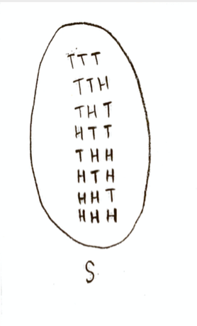
Let’s take our experiment to be flipping a coin three times. This is three Bernoulli trials; let’s call “success” getting a head, with probability 1/2. Then the sample space S is a set consisting of 8 points:
Let’s make our random variable be the number of successes. The book calls this random variable $\mathbf{S}_3$. It is a function on the sample space, whose input is a point of the sample space (the result of an experiment, e.g. “HTH”), and whose output is a natural number, the number of heads (successes) in that result. I would draw it conceptually like this:
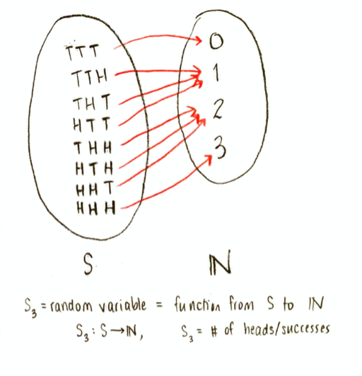
The co-domain of $\mathbf{S}_3$ is the set of natural numbers $\mathbb{N}$, and the range is the set of numbers $\{0,1,2,3\}$. (In this context, the co-domain is a somewhat arbitrary choice; I could have also thought of the co-domain as being the set $\mathbb{R}$ of real numbers. But the range would still be the set ${0,1,2,3}$.)
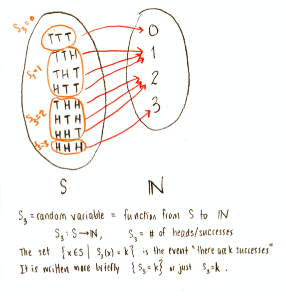
Now, any possible value of $\mathbf{S}_3$ defines an event. For example, the set $\{x\in S\vert \mathbf{S}_3(x)=2\}$ is the set of all points in the sample space such that $\mathbf{S}_3=2$, that is, it is the set $\{HHT, HTH, THH\}$. That is an event (also written $\{\mathbf{S}_3=2\}$, or even just $\mathbf{S}_3=2$, for short).
Now, as always, we can find the probability of any event, by adding up the probability of all the points which make it up. We can therefore compute the probabilities $P(\mathbf{S}_3=0)$, $P(\mathbf{S}_3=1)$, etc. Finding probabilities is itself a function:
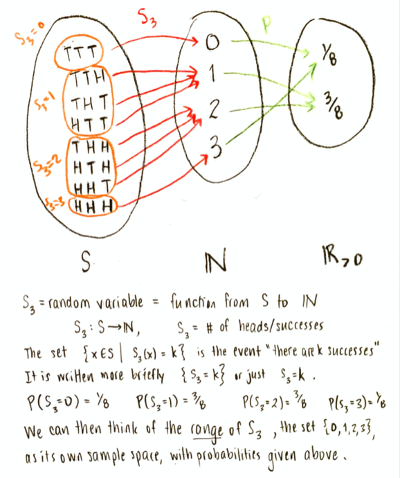
We call this new function the probability distribution of the random variable $\mathbf{S}_3$. It is a function f whose domain is the range of $\mathbf{S}_3$, and whose values are non-negative real numbers, defined by $f(k)=P(\mathbf{S}_3=k)$, for $k\in\{0,1,2,3\}$.
An important shift of viewpoint is that we could now think of the range of $\mathbf{S}_3$, the set $\{0,1,2,3\}$, as being a sample space in its own right, with the probabilities for the points being $P(\mathbf{S}_3=0)$, $P(\mathbf{S}_3=1)$, $P(\mathbf{S}_3=2)$, and $P(\mathbf{S}_3=3)$.
Note that we didn’t have to take the number of heads. We could have made many different random variables: we could have made chosen the number of tails, or the number of heads minus the number of tails, or the number of heads in the first two flips, or the number of heads squared, etc. What random variable we look at depends on the problem we are trying to solve.
Exercise 1: Suppose our sample space S is the set of outcomes of flipping a coin three times, as in the above example. Let X be the random variable on S whose value is “the number of heads in the first two flips”. Repeat all the steps I did above: draw the picture for the random variable X, find the corresponding events and probabilities.
Exercise 2: Go back to the sample space of putting three distinguishable balls into three cells, which was discussed in Chapter I, Section 2, Example (a), page 9. Make up a random variable for this situation (you could take the number of balls in cell 1, or the number of empty cells, or the number of occupied cells, or the maximum number of balls in a cell…). For your choice of random variable, start drawing the conceptual diagram like I did in the example above. It won’t be too tedious if you use the numbering from Table 1 on page 9 to identify the points, and if you group together points whose value of the random variable are the same. Be sure to make the final step of drawing the probability function as well.
Two examples: Page 213, paragraph after formula (1.2)
Note that the first part of this sentence is the example I wrote out (I wrote it for the case n=3 and p=0.5). Make sure you understand this statement; you should formulate a similar conceptual picture as before (at least in principle, you don’t have to draw it out explicitly).
The second half of the sentence (“whereas the number of trials…”) is a different example.
Exercise 3: What is the sample space for this example (“whereas the number of trials…”)? What is the random variable he is talking about? Draw a picture as we did before. Do you see where he is getting the probability distribution that he claims?
Joint Distributions: page 213 (from “Consider now two random variables…” up through and including page 215, example (a))
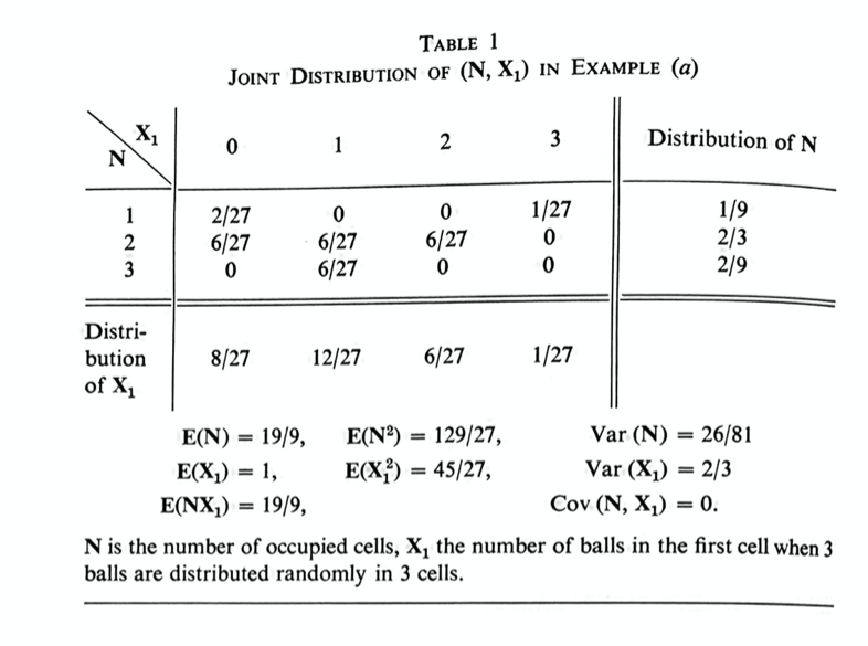
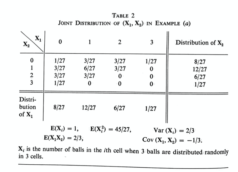
In order to understand this abstract idea of a joint probability distribution, it will be best to look carefully at an example. Helpfully, the author has given some very good examples on page 215, Example (a), and on page 214, Tables 1 and 2. I suggest working through these examples at the same time that you work through the abstract definitions; go back and forth, using the example to explain the definition, and identifying each part of the abstract definitions in the examples.
Don’t worry right now about the $\mathbf{E}(\mathbf{N})$ etc., at the bottom of Table 1 and Table 2; those are expectations and variances, which we will be getting to in the following sections.
Exercise 4: In this exercise, I am asking you to work through page 215, Example (a), and page 214, Tables 1 and 2, in detail. I think it is important to work through these examples carefully and in detail. A joint probability distribution is an abstract idea; understanding these tables in detail will make the abstract idea much easier to understand.
(a) For all 9 entries in the main part of Table 1, say what event the entry corresponds to, in words.
(b) Check every number in the main part of Table 1. You should be able to calculate yourself all 9 probabilities in the main part of this table. For each of the 9 probabilities, list the points in the corresponding event (use the numbering from page 9, Table 1).
(c) Check the marginal distributions of $\mathbf{N}$ and $\mathbf{X}_1$, on the side and bottom of this table. Check each number in two ways: (i) add up all the probabilities in that row or column, and (ii) calculate the probability directly. Compare the calculations you did in (i) and in (ii) in words (that is, say what the corresponding events are).
(d) Do all the same steps for at least some of Table 2. You don’t have to do every entry if it’s starting to feel repetitive, but you should at least spot-check the table, and convince yourself that you could do every entry, both the joint distributions and the marginal distributions.
Exercise 5: Let’s make our own joint distribution table. Suppose that we are flipping a coin three times. Let $\mathbf{X}$ be the random variable “total number of heads”, and let $\mathbf{Y}$ be the random variable “number of heads in the first two flips”. Make a joint distribution table, like in Tables 1 and 2 on page 214. Include the marginal distributions on the side and bottom. Check everything: make sure your probabilities in the main part of the table all add to 1; that the entries in each row add to the marginal distribution for one variable; and that the entries in each column add to the marginal distribution for the second variable.
Examples (b), (C), and (d), pages 215–217
I’m going to make a judgment call here: Example (b) on page 215 involves the multinomial distribution, which I skipped over earlier, so I’m going to skip it on first reading. Looking ahead, Example (d) on page 216 also involves the multinomial, so I will skip this on first reading as well.
(Example (d) turns out to be quite interesting, so I do want to come back to it. But I don’t want to get too bogged down the first time through. Remember that I am making suggestions here on how to read a text yourself—it’s often a good idea to skip over tough bits and come back to them. So, I’m going to come back to Examples (b) and (d), but I will put those later. In other words, I will write this lecture in the suggested reading order. I hope that does not prove to be too confusing!)
I will do Example (c) on page 216, because it is related to examples we have done in previous chapters, and it is seems like it will give a different type of example of a random variable and joint distribution.
Exercise 6: Let’s work through Example (c) on page 216. I am imagining the Bernoulli trials as coin flips, with heads a success. (However, I will keep the probability of a head general as p, and the probability of a tail as q=1-p, in order to keep things general.) We are playing a game where we flip the coin until we get a total of exactly two heads, and then we stop.
(a) Start writing out the points of the sample space. There are infinitely many, so you can’t write them all. But I found that trying to find a systematic way to list them helped me understand what all the possibilities are.
(b) What two numbers would tell you completely which point in the sample space you are at?
(c) What do the random variables $\mathbf{X}_1$ and $\mathbf{X}_2$ measure? Think about what they are for some of the points of the sample space you wrote out.
(d) Figure out the probabilities of some of the points you wrote in your sample space.
(e) Derive for yourself the formula that the author gives for the joint probability: $$P(\mathbf{X}_1=j,\mathbf{X}_2=k)=q^{j+k}p^2.$$ Check it on a few values of j and k to be sure that it works correctly.
(f) The author says, “summing over k we get the obvious geometric distribution for $\mathbf{X}_1$”. Let’s unpack and check this statement. “Summing over k” means finding $$\sum_{k=0}^\infty P(\mathbf{X}_1=j,\mathbf{X}_2=k) = \sum_{k=0}^\infty q^{j+k}p^2 = q^jp^2 + q^{j+1}p^2 + q^{j+2}p^2 +\dotsb$$ Say to yourself in words what each term means. Then say what the whole sum should add up to, in words (i.e. say what event the whole sum is the probability of). Now, use the sneaky trick for adding up infinite (geometric) sequences: let $$S = q^jp^2 + q^{j+1}p^2 + q^{j+2}p^2 +\dotsb,$$ multiply S by q to find qS, and subtract. Get a final answer for the sum. Check that it agrees with what the probability should be for the event it represents.
(g) What would a joint probability table look like for this problem? Write it out (some of it at least). Include the marginal probabilities.
Conditional Probabilities and Independence, page 217
Let’s read through the discussion of conditional probability distributions, dependence, and independence on page 217.
The author says, “A glance at tables 1 and 2 shows that the conditional probability (1.12) is in general different from $g(y_k)$.” Let’s do that.
Looking at Table 1, what does the first column (columns go up and down) mean? For all entries in that column, $\mathbf{X}_1=0$: there are no balls in the first cell. The first entry says $P(\{\mathbf{X}_1=0\}\cap\{\mathbf{N}=1\})=2/27$: there is a 2/27 chance that the first cell is empty, AND there is one occupied cell. To find the conditional probability, we have to do: $$P(\mathbf{N}=1\big\vert\mathbf{X}_1=0)=\frac{P(\{\mathbf{X}_1=0\}\cap\{\mathbf{N}=1\})}{P(\mathbf{X}_1=0)}.$$ We get $P(\mathbf{N}=1\big\vert\mathbf{X}_1=0)=(2/27)/(8/27)=1/4.$
Exercise 7:
(a) Do the same thing for $P(\mathbf{N}=2\big\vert\mathbf{X}_1=0)$ and for $P(\mathbf{N}=3\big\vert\mathbf{X}_1=0)$. Check that $P(\mathbf{N}=1\big\vert\mathbf{X}_1=0)+P(\mathbf{N}=2\big\vert\mathbf{X}_1=0)+P(\mathbf{N}=3\big\vert\mathbf{X}_1=0)=1.$
(b) Now, compare the probability distribution $g(k)=P(\mathbf{N}=k)$ (which is also on Table 1) with the conditional distribution $f(k)=P(\mathbf{N}=k\big\vert\mathbf{X}_1=0)$. Verify what the author says, that they aren’t the same. See how much you can intuitively understand the differences.
(b) Quickly do the same thing for the other three columns in Table 1. You can just do it mentally if it’s getting tedious to write. Be sure to say to yourself what the different entries mean.
(c) Do the same thing for the first row of Table 1. Again, you can just do it mentally if you want.
(d) Same thing (at least perfunctorily) for the remaining rows of Table 1.
(e) Look at (1.12) again. Identify the notation there with what you were just doing: i.e. what is $y_k$, what is $x_j$, what is $f(x_j)$, and so forth. Make sure you understand why (1.12) is true.
The author then gives examples of the “strongest degree of dependence” between $\mathbf{Y}$ and $\mathbf{X}$, when $\mathbf{Y}$ is a function of $\mathbf{X}$. Let’s check these:
Exercise 8: Suppose that we are flipping a coin three times.
(a) Let $\mathbf{X}$ be the number of heads, and let $\mathbf{Y}$ be the number of tails. Make the joint distribution table for $\mathbf{X}$ and $\mathbf{Y}.$ Is what the author says true about the joint distribution table?
(b) Let $\mathbf{X}$ be the number of heads, and let $\mathbf{Y}=\mathbf{X}^2.$ Make the joint distribution table for $\mathbf{X}$ and $\mathbf{Y}.$ Again, is what the author says true about the joint distribution table?
Then, the author talks about the case where $\mathbf{X}$ and $\mathbf{Y}$ are independent.
Exercise 9: How does (1.12) simplify when $\mathbf{X}$ and $\mathbf{Y}$ are independent? (Put $p(x_j,y_k)=f(x_j)g(y_k)$ into (1.12) and simplify.) What does this mean in words?
The author says that, when the two random variables are independent, “the joint distribution assumes the form of a multiplication table”. Let’s try to make an example where the variables are independent, so we can see what he means:
Exercise 10: Suppose we flip four coins. Let $\mathbf{X}$ be the number of heads in the first two flips, and let $\mathbf{Y}$ be the number of heads in the second two flips.
(a) Make the joint distribution table for $\mathbf{X}$ and $\mathbf{Y}$. Include the marginal distributions on the sides.
(b) Can you see what the author is saying about “the joint distribution assum[ing] the form of a multiplication table”?
(c) Repeat the above with a “generalized coin”: still assume we are flipping four coins, still make $\mathbf{X}$ and $\mathbf{Y}$ defined as before, but let the probability of a head be p and the probability of a tail be q (not necessarily p=q=1/2). Make the joint distribution table. Include the marginal distributions. Check that this does in fact make a multiplication table.
Exercise 11: In example (c) on page 216, look at the joint distribution table you made. Is it a multiplication table? Does that mean $\mathbf{X}_1$ and $\mathbf{X}_2$ are independent? Intuitively, would you expect $\mathbf{X}_1$ and $\mathbf{X}_2$ to be independent? Why or why not?
At the end of this passage, the author says, “for example, the two variables $\mathbf{X}_1$ and $\mathbf{X}_2$ in table 2 have the same distribution and are dependent”.
Exercise 12: Check this statement: how can you tell from just looking at the table that $\mathbf{X}_1$ and $\mathbf{X}_2$ are dependent? Pick one entry in the table, and compare the joint probability with what it would have been if $\mathbf{X}_1$ and $\mathbf{X}_2$ were independent. Can you say in words what that means about the dependence? Does that make intuitive sense?
Formal definitions (pages 217–218, starting at “definition” on the bottom of page 217 and going to example (e) on the bottom of page 218)
Hopefully, spending all this time working through particular numerical examples will make it easier to read and understand these general definitions and statements. If it gets too airy, try translating the statements back to specific examples.
Example (e) on page 218
This example is pretty easy, and the author doesn’t do anything with it right now, so it’s worth reading. Note that the classic binomial we have been doing is a special case of this example.
Discussion at the top of page 219 (before example (f))
The author is making the point that I did above and in class: that once you choose a random variable, figure out the possible values (range of function), and figure out the probabilities of those values, then you could forget about the original sample space entirely. This is often a useful point of view.
The author is saying that some people go further, and just don’t define the sample space in the first place! You could just start by defining random variables. The author says that this is logically actually a bit simpler, but is less concrete and can be confusing.
Example (f), page 219
The author is trying to give a concrete way of picturing probabilities here. I personally didn’t find it that helpful, but it’s worth trying it out once to see if you might find it helpful:
Exercise 13 (optional): Try doing the author’s construction in Example (f) for Table 1 on page 214. Subdivide a circle into 27 equal pieces. (Easier than it sounds: cut it into three, then each piece into three, then each of those pieces into three. You don’t have to be accurate.) Then mark pieces corresponding to each of the 9 entries in Table 1. (Some of the pieces will have length 0, so you could leave those out.) Then, the probabilities of a ball landing in these zones on this roulette wheel would be identical to the probabilities corresponding to balls in cells that you talked about with Table 1.
Example (g), page 219
Exercise 14: Find the probability distributions for $\mathbf{X}_1+\mathbf{X}_2$ and $\mathbf{X}_1\mathbf{X}_2$ from Table 1, and check the author’s numbers that he gives for these.
Example (h), pages 219–220
This goes back to Example (c).
Since it keeps coming up, I think it’s worthwhile at this moment to make an aside about geometric series once and for all:
ASIDE ON GEOMETRIC SERIES
A “geometric series” is a sequence of added terms, where you get each term by multiplying the previous term by a fixed value. Or, said differently, the ratio of any two terms is the same. For example, $$S=4+12+36+108+324$$ is a geometric series with first term 4, and common ratio (or multiplying factor) 3.
(The term “geometric” is for historical reasons; there isn’t anything particularly geometric about them.)
In general, if we start with a first term a, and get each following term by multiplying by a common ratio r, continuing for n terms, we get the geometric series $$S=a + ar + ar^2 + ar^3 + \dotsb + ar^{n-1}.$$ We can make a simplified formula for S by multiplying both sides by r, and subtracting S-rS so that most terms cancel: $$rS = ar + ar^2 + ar^3 + ar^4+ \dotsb + ar^{n},$$ so $$S-rS = a-ar^n=a\left(1-r^n\right),$$ and $$S=\frac{a\left(1-r^n\right)}{1-r}.$$ For this class, we often have the ratio $r$ being positive and less than 1. In general, if $\vert r\vert<1$, then as n gets larger and larger, $r^n$ gets smaller and smaller. So we can take the limit as $n\to\infty$, and get the infinite geometric series $$S=a + ar + ar^2 + ar^3 + \dotsb = \frac{a}{1-r}.$$ From now on, you can just use that formula without re-deriving it, if you want!
OK, now let’s return to Example (h). To make it concrete, it might help to imagine flipping a coin, as we did for Example (c). We can keep it general by imagining a “generalized coin”, with probability p of heads and q=1-p of tails.
Exercise 15:
(a) What does the random variable $\mathbf{S}$ mean in words?
(b) The author says, “to obtain $P(\mathbf{S}=\nu)$ [that’s a greek letter ‘nu’] we have to sum (1.9) over all values j, k such that $j+k=\nu$”. To make sense of a statement like that, I usually recommend starting with specific values. What’s the least $\nu$ could be? It could be $\nu=0$; what are the corresponding values of j and k? Make the sum. Say what each thing you are doing means in words at every step. Now do the same for $\nu=1$, $\nu=2$, $\nu=3$. Finally, write a formula for a general $\nu$.
(c) Check the author’s statement that “there are $\nu +1$ such pairs”.
(d) There are some bad typos in the next statement: the two formulas that follow are very messed up. Write the correct formulas, based on what you just did.
At this point, things are getting more specialized; I’m feeling like I could work out the thing about $\mathbf{U}$ and so on, but that it’s maybe more important to go on. I might come back to the rest of Example (h) if I have time.
Note on Pairwise Independence
Since this seems like a technical point, I will skip it for now, and perhaps come back to it on a second reading.
2. Expectations
The expectation of a variable is, roughly speaking, an average. This is explained in the first paragraph of the chapter:
First paragraph, pages 220–221
Exercise 16: The author says: “If in a certain population $n_k$ families have exactly k children, the total number of families is $n=n_0+n_1+n_2+\dotsb$ and the total number of children [is] $m=n_1 + 2n_2 + 3n_3 + \dotsb$. The average number of children per family is $m/n$.” It is worth it to expand on this a bit.
(a) Explain to yourself each of the three statements above.
(b) From the above, show that you can rewrite the average number of children per family as $$\frac{m}{n}=0\frac{n_0}{n}+1\frac{n_1}{n}+2\frac{n_2}{n}+3\frac{n_3}{n}+\dotsb$$
(c) Let $p_k$ be the probability that a family has k children, ($k=0,1,2,3,\dotsc$). Show that you can write the average number of children per family as $$\frac{m}{n}=0p_0 + 1 p_1 + 2p_2 + 3p_3 + \dotsb$$
Definition and discussion, page 221
In the exercise we just did, using summation notation, we can write the average number of children per family as $$\frac{m}{n}=\sum_{k=0}^\infty kp_k.$$ In that example, our random variable $\mathbf{X}$ was “number of children in the family”, and the acceptable values of the variable (range of the function $\mathbf{X}$) were non-negative integers, $\{0,1,2,3,\dotsc\}.$
More generally, the outputs of a random variable don’t have to be all non-negative integers. The text is writing the output values (range) of $\mathbf{X}$ as $\{x_0,x_1,x_2,x_3,\dotsc\}$, or $\{x_k\}$ for short. They are writing the probability that $\mathbf{X}$ takes values $x_k$ as $f(x_k)$. So when we rewrite the formula for average value we did in the previous example into more general terms, we get $$E(\mathbf{X})=\sum x_k f(x_k),$$ where the sum runs over all the possible values of $x_k$.
It is possible that there are infinitely many $x_k$ in the range of $\mathbf{X}$, in which case the formula for the expectation is an infinite series. In that case, we have to demand that the series converges to a finite value; that is, it should get closer and closer to some fixed number as we add more terms. If that doesn’t happen, we say the expectation is not defined in that case.
(In fact, we have to demand something stronger: if some of the $x_k$ are negative, it is actually necessary that the infinite sum $\sum \big\vert x_k\big\vert f(x_k)$ converges. This is a technical point from analysis. It becomes important when doing infinite sample spaces intensively, but it won’t be important for us right now.)
The paragraphs after the definition reinforce what we worked out before in the previous exercise, and mention some different notations.
Expectation of a function of a random variable: last paragraph of page 221 through theorem 1 on page 222
Suppose we have a random variable $\mathbf{X}$ whose values are real numbers. Given any real-valued function $\phi:\mathbb{R}\to\mathbb{R}$, we can make a new random variable $\phi(X)$.
For example, if we flip a coin 4 times, and $\mathbf{X}$ is the number of heads, we could also make random variables like $\mathbf{X}^2$, or $3\mathbf{X}^2-2\mathbf{X}+1$, or $\sin(\mathbf{X})$.
The discussion in the last paragraph of page 221 talks about a random variable which might have negative and positive values, so let’s make up an example where that is the case, to understand that paragraph:
Exercise 17: Suppose that we flip a coin 4 times. Let $\mathbf{X}$ be the number of heads minus the number of tails.
(a) List all the values $x_k$ that this random variable can have. List their probabilities. Calculate $E(\mathbf{X})$.
(b) List all the values that $\mathbf{X}^2$ can have.
(c) List the probabilities for each value of $\mathbf{X}^2$. (Be careful!)
(d) You can now find the expectation $E(\mathbf{X}^2)$ in two ways: you can sum over the three possible values of $\mathbf{X}^2$, or you can sum over the five possible values $x_k$ of $\mathbf{X}$. Write out both of those sums. Note that the latter option is (2.2).
Exercise 18: Explain to yourself (in words) why (2.3) (in Theorem 1 on page 222) is true.
Exercise 19: Theorem 1 on page 222 has a second part: the author says “For any constant a we have $E(a\mathbf{X})=aE(\mathbf{X})$”. Prove this last statement.
Note: I personally find it easier to prove things about formulas in summation notation if I expand them. Otherwise I get mixed up. So, rather than writing the neat-looking formula $$E(\mathbf{X})=\sum x_k f(x_k),$$ I think it is almost always safer to write the messier-looking, but more explicit formula $$E(\mathbf{X})=x_0 f(x_0) + x_1 f(x_1) + x_2 f(x_2) + \dotsb x_n f(x_n).$$ Of course, once you have done that, you can always revert to the more compact notation for a final version if you want to. This point will be particularly important with some proofs coming up.
Theorem 2 and discussion (page 222)
Theorem 2 is particularly important, and will be used all the time.
Exercise 20: Write out the proof of Theorem 2 yourself. In particular:
(a) For simplicity, let’s imagine that $\mathbf{X}$ has only two possible values $x_1$ and $x_2$, and $\mathbf{Y}$ has only two possible values $y_1$ and $y_2$. Write out $E(\mathbf{X})+E(\mathbf{Y})$; using (2.1), you should get $$E(\mathbf{X})+E(\mathbf{Y})=x_1 f(x_1) +x_2 f(x_2) +y_1 g(y_1) +y_2 g(y_2).$$ (b) Next, I want to write out $E(\mathbf{X}+\mathbf{Y})$. Note that the random variable $\mathbf{X}+\mathbf{Y}$ has four possible values in this situation. You should get $$\begin{split}E(\mathbf{X}+\mathbf{Y})&=(x_1+y_1)p(x_1,y_1)+(x_1+y_2)p(x_1,y_2)\\ &+ (x_2+y_1)p(x_2,y_1)+(x_2+y_2)p(x_2,y_2).\end{split}$$ (c) Try to figure out how those two formulas above must be equal. You will be using (1.12), and also Chapter V (1.8) (or at least the idea from that formula). It may help to write out the sum in (2.5) explicitly—again assuming that there are only $x_1$, $x_2$, $y_1$, and $y_2$—to see how the author is arguing this.
(d) When the proof says “the sum can therefore be rearranged to give . . .”, rewrite that summation notation explicitly as well, and show that you can in fact rearrange (2.5) to get that answer. (I wouldn’t worry about the comment about “absolute convergence”. It is important in the case where the sums are infinite; surprisingly, you cannot always rearrange an infinite sum and get the same answer. The reason for demanding “absolute” convergence in the definition is that this is the condition you need to make rearrangement of an infinite sum valid.)
(e) We only proved this for when $\mathbf{X}$ and $\mathbf{Y}$ each have only two output values. Can you see how the same thing will work if there are more output values (that is, a larger range for the indices j and k)? (You don’t have to write it all out explicitly, though if you are interested in writing proofs, you could do so.)
After the theorem, the author says “clearly, no corresponding theorem holds for products; for example, $E(\mathbf{X}^2)$ is generally different from $(E(\mathbf{X})^2$”. Is this clear? Let’s check it:
Exercise 21:
(a) Check the numbers on the numerical example that the author gives.
(b) (Optional but instructive) Write it out more generally: repeat what you wrote for the proof of Theorem 2, but instead of writing the sum of $E(\mathbf{X})$ and $E(\mathbf{Y})$, write out their product. Compare it to what you get for $E(\mathbf{XY})$. (You don’t have to write out all the terms of the products, which would get quite long; but if you write out the brackets, and imagine doing the multiplication, you can see how they will be different.)
Expectation of a product of independent variables: Theorem 3, pages 222–223
Exercise 22: Work through the proof of Theorem 3. Start with the same steps as I suggested for Theorem 2, except that you are writing the product rather than the sum. In particular, assume there are only $x_1$, $x_2$, $y_1$, and $y_2$. See if you can figure out how to prove $E(\mathbf{X}\mathbf{Y})=E(\mathbf{X})E(\mathbf{Y})$ from that. Write out (2.7) explicitly, to see how the author is arguing this.
Discussion of conditional expectation (paragraphs after Theorem 3 on page 223)
Note that the conditional expectation $E(\mathbf{Y}\big\vert \mathbf{X})$ has a sum over $y_k$, but not over $x_j$; it depends on $x_j$. So, for each value $x_j$ that $\mathbf{X}$ can take, the expression $E(\mathbf{Y}\big\vert \mathbf{X}=x_j)$ is a number. Since it outputs a number for each value of $x_j$, I can think of it as a random variable itself. That is, it is a function, whose input is the range of $\mathbf{X}$, that is, the set $\{x_0, x_1, x_2,\dotsc\}$, and whose output is a real number. So $E(\mathbf{Y}\big\vert \mathbf{X})$ is a random variable: the $\mathbf{Y}$ has been averaged over, but the $\mathbf{X}$ is still a free variable.
Exercise 22: Work out $E(\mathbf{N}\big\vert \mathbf{X_1})$ for Table 1 on Page 214. Note that “working it out” means that you will get a list of four numbers. Say to yourself in words what each of these numbers means. Make sure that the answers make intuitive sense (three of the four should be intuitively clear answers once you think about it the meaning).
(NUMERICAL ANSWERS: $E(\mathbf{N}\big\vert \mathbf{X_1}=0)=7/4$, $E(\mathbf{N}\big\vert \mathbf{X_1}=1)=2.5$, $E(\mathbf{N}\big\vert \mathbf{X_1}=2)=2$, $E(\mathbf{N}\big\vert \mathbf{X_1}=3)=1$.)
If we were being complete, I would try to prove (2.9) now, but let’s just move on!
3. Examples and Applications
This is where this chapter starts to get really cool. So far we’ve made a bunch of definitions. The surprising thing is that we can use the ideas of random variable and expectation (and later variance) to find interesting results about probabilistic situations, without actually calculating all the probabilities on the sample space. This means we can do certain things much more easily now.
I’ll cover some of the examples of this section now, and skip some over for now. They are all interesting, so I’ll come back to them on a second reading.
Example (a): The Binomial Distribution (page 223)
The author wants to prove the following important result: if $\mathbf{S}_n$ is the number of successes in n Bernoulli trials, with probability of success p (and probability of failure q), (so we have a binomial probability distribution for $\mathbf{S}_n$), then the expected value $\mu$ of $\mathbf{S}_n$ (expected average number of successes) is $$\mu=E(\mathbf{S}_n)=np.$$ This makes sense intuitively, but how to prove it? The author gives two methods, one harder way and one easier way. Let’s follow those:
Exercise 23: Proving that the expected value of the binomial distribution $b(k;n,p)$ is $np$:
(a) Hard way: Write out the formula for $b(k;n,p)$. In the formula, expand out the binomial coefficient. Now, write out the formula for $b(k-1;n-1,p)$. How are they different? They should only be different by a simple multiplicative factor. Use this to prove that $$b(k;n,p)=[\text{something}]b(k-1;n-1,p).$$ Now, the author starts out writing $$E(\mathbf{S}_n)=\sum kb(k;n,p);$$ why is this true? What index is the sum over, and what is the range of that index? Sub in the formula you worked out above to get the author’s second equality. Finally, he says that the last summation you get comes out to 1, why is that? In the end you should find $$E(\mathbf{S}_n)=np$$ as the author does.
(b) Easy way: I won’t add anything to the author’s argument here, but be sure you understand it. It’s important. And much easier than the first way!
Example (b): Poisson Distribution (page 224)
Here, the author is saying that $\mathbf{X}$ has a Poisson distribution. That is, $X$ is the number of events (e.g. raisins in a cookie, or stars in given area of sky), when the events (e.g. raisins or stars) are happening randomly.
The parameter $\lambda$ has to do with how frequent the events are. Previously, I argued intuitively that $\lambda$ corresponds to the average number of events per unit of time or space. Now we prove it: if $\mathbf{X}$ is a random variable, with output values $x_0=0$, $x_1=1$, $x_2=2$, . . . , $x_k=k$, and the probability $P(\mathbf{X}=k)$ is given by the Poisson distribution, $P(\mathbf{X}=k)=\dfrac{\lambda^k}{k!}e^{-\lambda},$ then the expected value of $\mathbf{X}$ is $$E(\mathbf{X})=\lambda.$$ Let’s follow the author’s proof:
Exercise 24: Similarly to the “hard way” for the binomial, write out the formula for both $p(k;\lambda)$, and for $p(k-1;lambda)$, where $p(k;\lambda)$ is the Poisson distribution. See how they are different; you should be able to find a formula of the form $$p(k;\lambda)=[\text{something}]p(k-1;\lambda).$$ Now, the author says $$E(\mathbf{X})=\sum k p(k;\lambda);$$ why is that true? What is the summation index here? What values does the summation index take? Now, substitute your formula into this one, to get (hopefully) the author’s second equality. He claims the sum in the last expression adds to 1; why? Finally, you should find $$E(\mathbf{X})=\lambda$$ as claimed!
Example (c): Negative Binomial Distribution (page 224)
The words “negative binomial distribution” are a little intimidating. And it does seem to refer to something we skipped over earlier. However, looking at the example, it actually seems to just be based on Example (c) of Section 1, which we did. So let’s try it!
(This example and Example (d) turn out to be good examples of how you can use random variables and expectations to easily solve something that would be quite hard otherwise.)
Example (c) seems to have three parts. I’ll talk about the first two parts in separate exercises, and skip the last part . . .
In the first 6 lines of Example (c), the author recalls the setup of Example (c) from Section 1 (page 216). (Read ahead to the fifth and sixth line for the interpretation.) Remember what we were doing there: flipping a coin repeatedly, tails = failure, and heads = success. We flip the coin until we get a success (head) and then stop. To keep things general, we leave the probability of a head to be p and the probability of a tail to be q=1-p (rather than setting them both to be 1/2). The author is working out the expected value of that distribution: that is, what is the expected number of tails we will flip before we get one head?
Exercise 25: (note the first few parts are repeating Example (c) in Section 1)
(a) We are flipping a coin repeatedly until we get the first head, and then we stop. What is the sample space for this situation?
(b) What is the probability for each of the points in the sample space you listed? (Leave them in terms of p and q; don’t set p=q=1/2.)
(c) Given what you worked out, make sure you understand the random variable $\mathbf{X}$ he describes, and the formula for its probability distribution $P(\mathbf{X})=q^k p$.
(d) Write out the formula for $E(\mathbf{X})$, which should simplify to the expression that he writes, $$E(\mathbf{X})=qp(1+2q+3q^2+4q^3+\dotsb).$$
(e) Now, he is finding the sum of the infinite series in brackets. There are two ways to do this; I’ll separate these out as another exercise below. The result is $$1+2q+3q^2+4q^3+\dotsb=\frac{1}{(1-q)^2}.$$ Taking this for granted for now, use it, and simplify, to obtain the final answer, $$E(\mathbf{X})=\frac{q}{p}.$$
(f) Before we leave this part, let’s think about what this means. We keep playing until we get one success. The expected number of failures before the first success is q/p. (i) What does this say for a normal coin, with p=1/2? What does that mean in words? (ii) Let’s say we are rolling a die, with rolling a “six” as success, and anything else as failure. What is $E(\mathbf{X})$? What does this mean in words? (iii) Let’s go back to the lottery example: suppose that the chance of winning is p=1/1,000,000. What is the expected number of losing tickets we will have to get before having one win?
Exercise 26: This exercise is explaining how to find the result $$1+2q+3q^2+4q^3+\dotsb=\frac{1}{(1-q)^2}$$ that we just used. Note that the formula for a geometric series doesn’t work directly, because this is not a geometric series. There are two ways to find this sum:
(a) Let $S=1+2q+3q^2+4q^3+\dotsb$. Using a similar trick as before, find $qS$, and then find $S-qS$. You will have infinitely many terms that don’t cancel—but those terms will form a series that you can find the sum of. Put in the formula for the sum, and solve for $S$.
(b) If you happen to know calculus, you can start with the sum of the infinite geometric series: $$1+ q + q^2 + q^3 + q^4 = \frac{1}{1-q},$$ and take the derivative of both sides! (This is the method the book alludes to.)
Next, the book talks about continuing this game until the nth success. So in our example, we are flipping the coin until we get n heads.
In understanding what’s written for a general n, it’s always a good idea to start with specific values. What we did above was n=1, so let’s try n=2.
Exercise 27: Suppose n=2 in the discussion in the second half of Example (c).
(a) What are the points of the sample space? What determines a point of the sample space?
(b) I think the author should have had $r\leq n$ (rather than $r<n$). For r=1, what is $\mathbf{X}_1$? For r=2, what is $\mathbf{X}_2$? What are the possible output values of $\mathbf{X}_1$ and $\mathbf{X}_2$? Say what $\mathbf{X}_1$ and $\mathbf{X}_2$ are for several of the points you listed in the sample space.
(c) Intepret the random variable $\mathbf{Y}=\mathbf{X}_1+\mathbf{X}_2$. What are the possible output values of $\mathbf{Y}$?
(d) How many points are in the event $\{\mathbf{Y}=0\}$? What is its probability?
(e) How many points are in the event $\{\mathbf{Y}=1\}$? What is its probability?
(f) How many points are in the event $\{\mathbf{Y}=2\}$? What is its probability?
(g) Figuring out the probabilities for $\mathbf{Y}$ is going to be a little bit involved. It is possible, but that is the thing we skipped over in Chapter VI, Section 8. However, it is much easier to find its expectation, even without knowing its probability distribution. We can use Theorem 2, as the author says. What is $E(\mathbf{Y})$? (Remember we are fixing $r=2$, so $\mathbf{Y}=\mathbf{X}_1+\mathbf{X}_2$.) Find this numerically in the examples of flipping a coin, rolling a die (with “six” success), and playing a p=1/1,000,000 lottery, and interpret the answer in words in each case.
(h) Suppose now that $r=3$, so $\mathbf{Y}=\mathbf{X}_1+\mathbf{X}_2+\mathbf{X}_3$. Find how many sample points are in the event $\{\mathbf{Y}=2\}$, for example. I ask this just to illustrate that finding the distribution of $\mathbf{Y}$ is going to be tricky for general r! (You can find the answer in Chapter VI Section 8 if you’re interested.) But you can find the expectation very easily. For example, find it in the case of coin flips, and interpret.
The last part of Example (c) talks about how to do this problem the “hard way”, using the probability distribution of $\mathbf{Y}$ that was worked out in Chapter VI, Section 8. But I’m not going to worry about that.
Example (d): Waiting times in sampling (pages 224–225)
This example is very interesting practically and theoretically. It is based on Example (c) above. I have run out of time to give you guidance on this, but I strongly recommend working through Example (d)! I will update this next time with more guidance.
What next?
I’ve run out of time for the moment. I’ll update this more soon, and let you know when I have.
In the meanwhile, I would recommend working through Example (d), and then perhaps skipping Examples (e) and (f) for now. Skip ahead to Section 4: Variance, and work through that section carefully as you have the previous ones. Everything in that section is important.
Section 5 is also quite important, and contains some more examples of powerful things you can figure out with these methods. In that section, I recommend working through the Definition and Theorems, and studying Examples (a), (b), and (c), but perhaps leaving (d) for a second reading.
We will skip Sections 6 and 7.
Section 8 is worth doing, because the correlation coefficient comes up all over the place. I will talk about this in class as well.
Sorry for the delays, and I’ll see you in class!