
Hi everyone!
OK, I had planned to go in strict logical order from now on, but I just couldn’t do it. I was too worried about 1) running out of time for important things, and 2) taking away emphasis from the central ideas.
So what I’m going to do is start with a key example. Then I’ll talk about theory backing that up, and then a new example, and so on. I am planning to write the foundational lectures still, as we go. But I think this way will make more sense (though I know it doesn’t sound like it from what I just said!).
OK, let’s get started.
Eigenvalues, eigenvectors, and spectral decomposition
First, just a little bit of context and theory. I am not going to use this right away in the example, but this is where I’m heading.
Suppose we have linear transformation $A$ that maps a vector space back to itself, $A:V\to V$. It is interesting to know, in many applications, if $A$ has a fixed point: some vector $\vec{v}\in V$ such that
$A\vec{v}=\vec{v}$.
In fact, a more general thing is often of interest: whether $A$ has an invariant line. A line through origin $L$ would be called invariant if:
for any vector $\vec{v}\in L$, we also have $A\vec{v}\in L$.
A line through the origin is a 1-dimensional subspace, so such a fixed or invariant line is usually called an invariant 1-dimensional subspace.
You should take a moment to convince yourself that $A$ has an invariant line $L$ exactly when there exists a non-zero vector $\vec{v}_0$ with the property that
$A\vec{v}_0 = \lambda \vec{v}_0$, for some scalar $\lambda$.
Understanding Exercise: Eigenvectors and Invariant Lines
Give a rough explanation (to yourself is fine, you don’t have to write it out necesssarily) of the statement above: that $A$ has an invariant line exactly when there is a non-zero vector $\vec{v}_0$ with the stated property. It doesn’t have to be a precise proof (see below).
Such a vector $\vec{v}_0$ is called an eigenvector, and the corresponding scalar $\lambda$ is called an eigenvalue. “Eigen” is German for “proper”, in the sense of “belonging to” (like “property”). In some older texts, eigenvectors are called proper vectors, or characteristic vectors. They are vectors which “belong to” or are “characteristic of” the transformation $A$.
Theory Problem: Eigenvectors and Invariant 1-D Subspaces
Suppose that $A:V\to V$ is a linear transformation as discussed above. Prove the following: if there exists an eigenvector $\vec{v}_0$ for $A$, then the line $L=\mathrm{span}\{\vec{v}_0\}$ is an invariant line (1-D subspace) for $A$. On the other hand, if $L$ is an invariant line for $A$, then any non-zero vector in that line is an eigenvector (and all the vectors in that line share the same eigenvalue).
This simple looking concept ends up being deeply useful in many contexts. Let me get into the examples first, and then I’ll come back to how the eigenvectors play a role in the examples. (In a later lecture, I’ll talk about how eigenvectors and eigenvalues are deeply theoretically important as well.)
A Markov chain: setting up the model
OK, here is an applied example, versions of which show up in all kinds of places (economics, physics, probability, computer science…).
Let’s suppose that we have some sort of system where agents can be in two states, let’s call them states 1 and 2. At time 0, we have a bunch of agents in state 1 and a bunch of agents in state 2. Then, in each time step, some proportion of the agents will flip states.
This setup could be used for demographics and economics: for example, state 1 could be urban residents and state 2 rural residents; each year some proportion move from on state to the other. For another example, in physics, an ammonia molecule can be in one of two main energy states, and its flipping back and forth is responsible for being able to create an “ammonia maser”.
Of course, there’s no limitation on the number of states, but I’m starting with just two states so that things are simple to write down.
Let’s use $x_j(t)$ to denote the number of agents in state $j$ at time $t$. So we start with $x_1(0)$ agents in state 1 and $x_2(0)$ agents in state 2.
Now, let me pick some numbers (arbitrarily). Let’s say that, in each time step, a proportion $0.10$ (that is, 10%) of the agents in state 1 move to state 2, and in each time step, a proportion $0.05$ (that is, 5%) of the agents in state 2 move to state 1.
We can illustrate the situation as follows:
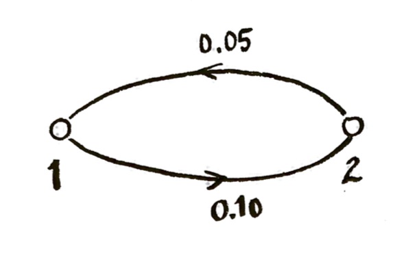
This picture is called a “directed graph” (not to be confused with “graph” like “graph of a function”). That states are called “vertices” or “nodes”, and the lines between the states are called “edges”. If we had more states, we would have a bigger directed graph.
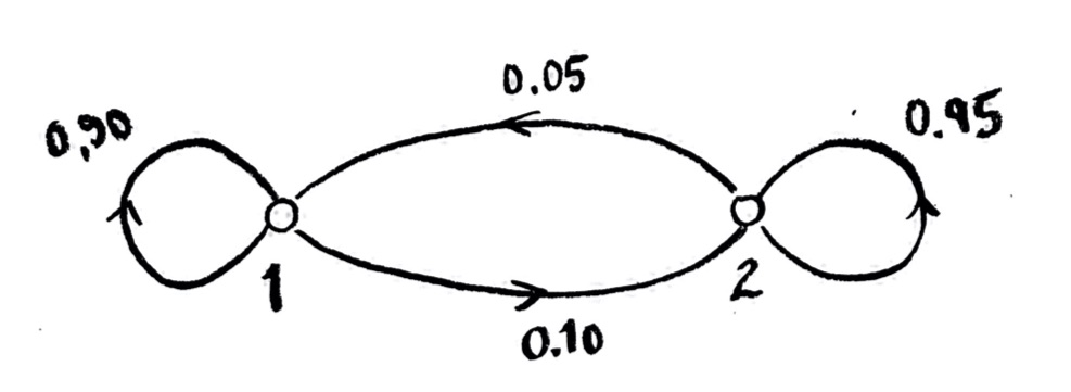
Sometimes people will also indicate the proportions which stay in the state they were in during each time step. Since 10% of the agents in state 1 leave in each time step, 90% of them stay, and similarly for state 2. We could draw it like this:
Note that the number of agents are conserved: agents are not born or killed. We could consider models where that happens, too! But the class of models where the number of agents is conserved are the ones I’ll consider first. These are called “Markov chains”.
It is maybe worth mentioning that, instead of having a bunch of agents, I could also just have one agent, who, each time step, randomly either switches states or stays in its state. Then I would make $x_1(t)$ and $x_2(t)$ be the probabilities that the agent is in state 1 or 2, respectively, at time $t$. You could also imagine this as an agent randomly walking around on a graph, according to assigned probabilities.
A Markov chain: setting up the equations
Alright, now that I’ve told you the assumptions, let’s set up the equations.
Understanding Exercise: Setting up Markov chain equations
Before you read on, try this yourself. Let’s say the time steps are $t=0,1,2,\dotsc$. Write the equations for $x_1(t+1)$ and $x_2(t+1)$ in terms of $x_1(t)$ and $x_2(t)$, with the assumptions about probabilities that I made above. Once you have the equations, try to rewrite them in matrix form.
Got it?
Here’s the answer in linear equations form:
$x_1(t+1)= (0.90) x_1(t) + (0.05) x_2(t)$
$x_2(t+1)= (0.10) x_1(t) + (0.95) x_2(t)$
In matrix form, we could write this as
$\begin{bmatrix}x_1\\x_2\end{bmatrix}(t+1)=\begin{bmatrix}0.90&0.05\\0.10&0.95\end{bmatrix}\begin{bmatrix}x_1\\x_2\end{bmatrix}(t)$
The matrix here,
$T=\begin{bmatrix}0.90&0.05\\0.10&0.95\end{bmatrix}$
is called the transition matrix.
It is often useful, in the equation, to separate out the number of agents from the previous time step, plus the change during the time step. That is, I would rewrite the equation above as
$\begin{bmatrix}x_1\\x_2\end{bmatrix}(t+1)=\begin{bmatrix}x_1\\x_2\end{bmatrix}(t)+\begin{bmatrix}-0.10&0.05\\0.10&-0.05\end{bmatrix}\begin{bmatrix}x_1\\x_2\end{bmatrix}(t)$,
which I could simplify as
$\begin{bmatrix}x_1\\x_2\end{bmatrix}(t+1)=\left(I+\begin{bmatrix}-0.10&0.05\\0.10&-0.05\end{bmatrix}\right)\begin{bmatrix}x_1\\x_2\end{bmatrix}(t)$,
where $I=\begin{bmatrix}1&0\\0&1\end{bmatrix}$ is the $2\times 2$ identity matrix.
Understanding Exercise:
Check that my rewriting of the equation is the same as the original (if I did it correctly!), and make sure you understand the meaning of the terms.
In this case, we would call the matrix which gives the changes in each time step,
$\Delta=\begin{bmatrix}-0.10&0.05\\0.10&-0.05\end{bmatrix}$,
the “difference matrix” or weighted graph Laplacian. Then,
$T=I+\Delta$.
A Markov chain: questions
Given these equations, we could start with any initial number of agents $x_1(0)$ and $x_2(0)$ in the two states 1 and 2, and see how they evolve over time. This would be a little tedious to do by hand, but easy enough with a computer.
One initial thing we might want to know is: does the system approach a steady state, i.e. an equilibrium? That is, do the numbers $x_1(t)$ and $x_2(t)$ settle down over time? Or do they oscillate forever?
Computing Problem: Two-State Markov Chain Example
For those of you who are interested in computing things, this would be a good example to start with. You probably have a preferred system for doing matrix computations already; if you don’t, you might try https://www.sagemath.org/, which combines Python with a Maple-like front end. Try some arbitrary starting values $x_1(0)$ and $x_2(0)$, and then find $x_1(t)$ and $x_2(t)$ for $t=1,2,3,\dotsc$. In particular, find these for fairly large values of $t$: do they in fact settle down, or do they oscillate? Try experimenting with the initial values: how does the behavior depend on what initial values you take?
If you do decide to do this computing exercise, you might want to try it before trying for theoretical answers in the next exercise:
Problem: Finding Two-State Markov Chain Steady State
a) Try to set up equations to determine if this two-state Markov system has a steady state. Assume the same probabilities as above. You might also want to assume some specific numerical values for $x_1(0)$ and $x_2(0)$, at least at first.
b) Try to solve for the steady state. Does the system have a steady state? If it does, check your answer!
c) How does your answer depend on the initial values $x_1(0)$ and $x_2(0)$? If you picked specific numerical values at first, try doing it with unspecified variables instead. Does the nature of the solution depend on the initial values?
c) Can you explain how this question is related to eigenvectors and eigenvalues?
Theory Problem: General Two-State Markov Chains
For those of you who are more theoretically inclined:
a) Do the previous problem, still with two states, but with general transition probabilities replacing the specific ones that I gave in my example. Give a general answer in terms of variables.
b) Can you prove when the system will have a steady state? Can you give a proof which would generalize to more than two states?
We might be interested, not only in the existence and nature of a steady state, but also how the system approaches a steady state. If you’ve done the other problems, here’s a challenge problem to think about: the state of the system at time $t=n$ is going to be given by
$\begin{bmatrix}x_1\\x_2\end{bmatrix}(n)=T^n\begin{bmatrix}x_1\\x_2\end{bmatrix}(0)$.
Can you use what we’ve done above, to find a simpler way of computing $T^n$, so that you can simply find out the state of the system for large time, without having to do a huge number of matrix multiplications?
More answers and explanations next time!