
Hello again!
I left off the last lecture (Eigenvalues II: Markov processes continued), not so much at a logical stopping point, but just where I got tired and ran out of time! A bit like ordinary class I guess.
In the last lecture, I showed how to
- change basis (coordinates) for a vector
- change basis (coordinates) for a linear transformation
- use a basis made of eigenvectors to simply compute powers of a matrix (applied to the transition matrix for our Markov example)
- use a basis made of eigenvectors to put the matrix of a transformation into simple (diagonal) form
- apply that diagonalization to again simply compute powers of a matrix (this time in matrix form)
At the end of that lecture, I started to show how to use the eigenvectors to decompose the matrix in a different way: as a sum of simple 1-D projection operators (tensor products of vectors and dual vectors). However, I didn’t get very far: I just reminded you about dual vectors, and computed them in our example.
In this lecture, I am going to show how the spectral decomposition works, and apply it to our example.
There is one thing I haven’t told you: how to actually FIND the eigenvectors! I’m going to put that off for a little bit: first I want to show you, in the last lecture and this one, how they are used mathematically (for diagonalization and spectral decomposition), and then in the next lecture to show you some more applications.
OK, let’s get started.
Reminder of our example from last time
To start, I am going to repeat what I said at the end of the previous lecture, for reference.
Recall that our main example was the following two-state Markov chain:
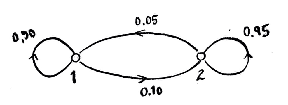
If $x_1$ and $x_2$ are the numbers of agents (or amounts of stuff, or probabilities of one agent) in the two states, then the system state vector $\vec{x}_n=\begin{bmatrix}x_1\\x_2\end{bmatrix}_n$ evolves from time state $t=n$ to $t=n+1$ by the evolution equation
$\vec{x}_{n+1}=T\vec{x}_n = (I+\Delta)\vec{x}_n$.
(I have switched from writing $\begin{bmatrix}x_1\\x_2\end{bmatrix}(t)$, from the last lecture, to $\begin{bmatrix}x_1\\x_2\end{bmatrix}_t$ instead. The former makes sense logically, because the vector is a function of time; however, most people write this the latter way, so it doesn’t get confused with multiplying by t. I’ll stick with the subscript from now on, but it is only a change of notation.)
In our example, the transition operator $T$ is given by the matrix in the $B=\left\lbrace\begin{bmatrix}1\\0\end{bmatrix},\begin{bmatrix}0\\1\end{bmatrix}\right\rbrace$ basis
$[T]_B=\begin{bmatrix}0.90&0.05\\0.10&0.95\end{bmatrix}$,
and the difference operator, or weighted Laplacian, $\Delta$, is given by the matrix
$[\Delta]_B=\begin{bmatrix}-0.10&0.05\\0.10&-0.05\end{bmatrix}$.
Reminder of our analysis so far
We used eigenvectors to better understand the behavior of this system.
The operator $T$ has eigenvectors $\vec{e}’_1=\begin{bmatrix}\frac{1}{3}\\\frac{2}{3}\end{bmatrix}_B$ and $\vec{e}’_2=\begin{bmatrix}1\\-1\end{bmatrix}_B$, with eigenvalues $\lambda_1=1$ and $\lambda_2=0.85$, respectively. The operator $\Delta$ has the same eigenvectors, with eigenvalues $\mu_1=0$ and $\mu_2=-0.15$ respectively.
We showed how to find the first eigenvector, but I did not show you yet how to find the second one. However, once you are given $\vec{e}’_1$ and $\vec{e}’_2$, it is easy to check that they are eigenvectors, and to find the corresponding eigenvalues.
(I could have equally well taken any non-zero scalar multiple of $\vec{e}’_1$ and/or $\vec{e}’_2$, and they would still be eigenvectors, with the same eigenvalues. I picked these particular multiples to make most sense with our example.)
The eigenvectors form a basis, $B’=\left\lbrace\vec{e}’_1,\vec{e}’_2\right\rbrace$. These are also called normal modes for the system.
If I can write my initial conditions in terms of the normal modes, then I can easily compute the operation of $T$ to any power. If my initial condition $\vec{v}_0=\begin{bmatrix}x_1\\x_2\end{bmatrix}_{B\ 0}$ can be written as $\vec{v}_0=x’_1(0)\vec{e}’_1 + x’_2(0)\vec{e}’_2$, then
$T\vec{v}_0=\lambda_1 x’_1(0)\vec{e}’_1+\lambda_2 x’_2(0)\vec{e}’_2$,
so
$T^nvec{v}_0=\lambda_1 ^n x’_1(0)\vec{e}’_1+\lambda_2^n x’_2(0)\vec{e}’_2=1 ^n x’_1(0)\vec{e}’_1+(0.85)^n x’_2(0)\vec{e}’_2$.
We can also so this computation in matrix form. We have the change of coordinate formulas
$[\vec{v}]_{B}=S[\vec{v}]_{B’}$
$[\vec{v}]_{B’}=S^{-1}[\vec{v}]_{B}$,
where $S$ is the change of coordinate matrix, whose columns are the $B’$ basis vectors, expressed in the $B$ basis. In our example,
$S=\begin{bmatrix}\frac{1}{3} & 1 \\\frac{2}{3} & -1\end{bmatrix}$, $S^{-1}=\begin{bmatrix}1&1\\\frac{2}{3} &-\frac{1}{3}\end{bmatrix}$.
We then have the change of coordinate formulas for linear operators,
$[T]_{B’}=S^{-1} [T]_B S$
$[T]_B=S [T]_{B’} S^{-1}$.
In our example,
$[T]_{B’}=\begin{bmatrix}\lambda_1&0\\0&\lambda_2\end{bmatrix}\begin{bmatrix}1&0\\0&0.85\end{bmatrix}$, $[\Delta]_{B’}=\begin{bmatrix}\mu_1&0\\0&\mu_2\end{bmatrix}=\begin{bmatrix}0&0\\0&-0.15\end{bmatrix}$,
and
$[T]_B=S\begin{bmatrix}\lambda_1&0\\0&\lambda_2\end{bmatrix}S^{-1}=\begin{bmatrix}\frac{1}{3} & 1\\\frac{2}{3} & -1\end{bmatrix}\begin{bmatrix}1&0\\0&0.85\end{bmatrix}\begin{bmatrix}1&1\\\frac{2}{3} &-\frac{1}{3}\end{bmatrix}$.
This diagonalization has some nice properties, one of which is that we can easily compute any power of $T$ in the ordinary $B$ basis:
$[T^n]_B=S\begin{bmatrix}\lambda_1^n&0\\0&\lambda_2^n\end{bmatrix}S^{-1}=\begin{bmatrix}\frac{1}{3} & 1\\\frac{2}{3} & -1\end{bmatrix}\begin{bmatrix}1^n&0\\0&(0.85)^n\end{bmatrix}\begin{bmatrix}1&1\\\frac{2}{3} &-\frac{1}{3}\end{bmatrix}$,
and similarly for $\Delta$.
Dual vectors
We have identified that the transition matrix $T$ has a steady-state vector ${\vec{e}’}_1$ given by
${\vec{e}’}_1=\begin{bmatrix}\frac{1}{3}\\\frac{2}{3}\end{bmatrix}$.
That is, the vector stays the same when $T$ is applied to it. (We could have equally well taken any non-zero scalar multiple of ${\vec{e}’}_1$, and that would also be fixed.)
We also mentioned that the total number of agents (or total probability) is fixed: the value
$x’_1=x_1+x_2$
is a constant. This is also a fixed thing, like the fixed/steady-state vector! But it is a different kind of thing: the fixed vector is a vector. This fixed thing $x’_1$ isn’t a vector; it’s a coordinate. More formally, it is a dual vector. And it is fixed, so it is an eigen dual vector. That’s hard to say, so we’ll say dual eigenvector instead.
Given some vector $\vec{v}=\begin{bmatrix}x_1\\x_2\end{bmatrix}_B$, how do I actually find its $x’_1$ and $x’_2$ coordinates? These are found by the dual vectors!
Recall that dual vectors are linear functions $f:V\to k$, whatever our field $k$ is. If they are written as matrices, and $V$ has dimension $n$, then they are $1\times n$ matrices. For this reason, they are also called row vectors.
Recall that the dual basis vectors $\overleftarrow{\phi}’_i$, $i=1,\dotsc,n$, corresponding to the basis $B’=\left\lbrace\vec{v}_i\right\rbrace$, $i=1,\dotsc,n$, are defined by being dual vectors satisfying the condition
$\overleftarrow{\phi}’_i\left({\vec{e}’}_j\right)=\begin{cases}1&i=j\\0&i\neq j\end{cases}$.
It’s not obvious that such dual vectors will always exist for any basis. I’ll ask that as a theory question in the next set of problems.
Assuming there exist these dual vectors, then they are the coordinate functions in the new basis! That is, if we have a vector $\vec{v}$, and it can be written in the new basis as $\vec{v}=x’_1\vec{e’}_1+x’_2\vec{e’}_2+\dotsb x’_n\vec{e’}_n$, then
For $i=1,\dotsc,n$, we have $x’_i=\overleftarrow{\phi}’_i(\vec{v})$.
Understanding exercise: Dual vectors give coordinates
Prove the above statement.
In our two-dimensional example, the $B’$ coordinates of any state vector $\vec{v}$ are given by $x’_1=\overleftarrow{\phi}’_1(\vec{v})$ and $x’_2=\overleftarrow{\phi}’_2(\vec{v})$.
How do I actually find the dual vectors? That is, how do I give their matrices in ordinary $B$ coordinates?
As a practical matter, you can use the defining conditions on the dual basis to set up linear equations for the matrices for the dual vectors, and solve. However, the dual basis matrices are actually already hidden in the change of coordinate matrices $S$ and $S^{-1}$ that we just talked about!
I claim that
the rows of $S$ are the matrices of the $B$ dual vectors, expressed in $B’$ coordinates, i.e. the $i$th row of $S$ is $[\overleftarrow{\phi}_i]_{B’}$,
and consequently that
the rows of $S^{-1}$ are the matrices of the $B’$ dual vectors, expressed in $B$ coordinates, i.e. the $i$th row of $S^{-1}$ is $[\overleftarrow{\phi}’_i]_{B}$.
This last thing is what we wanted. So, if we recall that
$S^{-1}=\begin{bmatrix}1&1\\\frac{2}{3} &-\frac{1}{3}\end{bmatrix}$,
we find that the dual vectors $\overleftarrow{\phi}’_1$ and $\overleftarrow{\phi}’_2$ have bases in the regular $B$ basis given by
$[\overleftarrow{\phi}’_1]_B=\begin{bmatrix}1&1\end{bmatrix}_B$
and
$[\overleftarrow{\phi}’_2]_B=\begin{bmatrix}\frac{2}{3} &-\frac{1}{3}\end{bmatrix}_B$ .
Understanding exercise: Computing coordinates with dual basis vectors
Check that this circle of ideas all closes up with a numerical example. Pick some numerical vector $\vec{v}=\begin{bmatrix}x_1\\x_2\end{bmatrix}$. Use the dual vectors above to find its $x’_1$ and $x’_2$ coordinates. Then check, in ordinary $B$ coordinates, that your chosen vector is in fact that linear combination of the $B’$ basis vectors: that is, check that $\vec{v}=x’_1\vec{e}’_1+x’_2\vec{e}’_2$.
Understanding exercise: Finding dual basis vectors from the change of coordinate matrix
a) See if you can explain why the statement I made is true: that the rows of the change of coordinate matrix $S$ are the matrices of the $B$ dual basis vectors, written in the $B’$ coordinates. To do this, you’ll have to think conceptually about what everything means. (I’m not looking for a formal proof here; I’ll ask that as a theory problem in a little bit. I’m just looking for a reason.)
b) Explain why that means that the rows of $S^{-1}$ are the matrices of the $B’$ dual basis vectors, written in the $B$ coordinates. (Which is usually what we want to find.)
In fact, we can write down change of coordinate formulas for dual vectors. If $f:V\to k$ is any dual vector, and if $S$ is the same change of coordinate matrix that we defined earlier (whose columns are the $B’$ basis vectors written in the $B$ basis), then
$[f]_{B’}=[f]_B S$, and
$[f]_B=[f]_{B’} S^{-1}$.
Understanding exercise: Change of coordinates for dual vectors
a) Try to explain to yourself why these formulas must be correct. (I’ll ask for a more formal proof later, but you could try to give one now if you’re interested.)
b) Use these formulas to solve the previous exercise. (Hint: what are the matrices $[\overleftarrow{\phi}_1]_B$ and $[\overleftarrow{\phi}_2]_B$? What are the matrices $[\overleftarrow{\phi}’_1]_{B’}$ and $[\overleftarrow{\phi}’_1]_{B’}$?
The spectral decomposition
Let’s look again at our example operator $T$. Using the eigenbasis $B’$, we can describe the action of $T$ as follows:
$T\vec{v}=\lambda_1 x’_1\vec{e}’_1+\lambda_2 x’_2\vec{e}’_2$.
That is, given any vector $\vec{v}$, we can calculate $T\vec{v}$ as follows:
- find the $x’_1$ and $x’_2$ coordinates of the vector $\vec{v}$;
- multiply the $x’_1$ coordinate by the corresponding basis vector $\vec{e}’_1$, and multiply that result by the eigenvalue $\lambda_1$;
- do the same for the second coordinate;
- and finally, add the results.
Well, we can write the instruction “find the $x’_1$ coordinate of $\vec{v}$” as a formula now! It is
$x’_1=\overleftarrow{\phi}’_1(\vec{v})$,
and similarly for $x’_2$. Consequently, we can write the recipe above as a formula: for any vector $\vec{v}$, we have
$T\vec{v}=\lambda_1 \overleftarrow{\phi}’_1(\vec{v})\vec{e}’_1+\lambda_2 \overleftarrow{\phi}’_2(\vec{v})\vec{e}’_2$.
I want to write this as an operator formula; that is, I want to leave out the “$\vec{v}$” in the formula. So I could write something like
$T=\lambda_1 \overleftarrow{\phi}’_1(-)\vec{e}’_1+\lambda_2 \overleftarrow{\phi}’_2(-)\vec{e}’_2$,
where the blank “$-$” is supposed to represent where I substitute in the argument $\vec{v}$. This is an odd way to write a function. So I define the notation $\vec{e}’_1\otimes\overleftarrow{\phi}’_1$. This thing is defined to be a linear function, which takes an input in $V$ and an output in $V$. It is defined to operate on an input $\vec{v}$ as follows:
$\vec{e}’_1\otimes\overleftarrow{\phi}’_1(\vec{v}):=\overleftarrow{\phi}’_1(\vec{v})\vec{e}’_1$.
Note that the output is a vector, so it is indeed a linear function from $V$ to $V$. It is called the tensor product, or outer product, of $\vec{e}’_1$ and $\overleftarrow{\phi}’_1$.
Using this notation, I can write
$T=\lambda_1 \vec{e}’_1\otimes\overleftarrow{\phi}’_1+\lambda_2 \vec{e}’_2\otimes\overleftarrow{\phi}’_2$.
This is called the spectral decomposition of the operator $T$. (The set of eigenvalues of the operator are called its spectrum. This is because the spectral lines in chemistry are computed by means of eigenvalues of an operator (a story for next term!).)
What does the spectral decomposition mean?
What kind of a thing is $\vec{e}’_i\otimes\overleftarrow{\phi}’_i$. First I want to describe it conceptually, and then explicitly in coordinates.
Conceptually, any vector $\vec{v}$ can be written as a linear combination of vectors in the $B’$ basis,
$\vec{v}=x’_1\vec{e}’_1+\dotsb+x’_n\vec{e}’_n$.
Let’s look at the meaning of the first coordinate. In the language we introduced earlier, the vector space $V$ is direct sum of the subspaces $V_1=\mathrm{span}\lbrace\vec{e}’_1\rbrace$ and $V’=\mathrm{span}\lbrace\vec{e}’_2,\dotsc\vec{e}’_n\rbrace$. The projection of a vector $\vec{v}$ onto $V_1$, along $V’$, is, by definition, $P_{V_1}^{V’}(\vec{v})=x_1\vec{e}’_1$.
The $x’_1$ is the first coordinate of $\vec{v}$ in the $B’$ basis; the product $x’_1\vec{e}’_1$ is the (vector) projection of $\vec{v}$ onto that first coordinate axis, along all the other coordinate axes.
Therefore, the tensor product $\vec{e}’_1\otimes\overleftarrow{\phi}’_1$ is a projection operator! It is the projection $P_{V_1}^{V’}$, where $V_1$ and $V’$ are defined as above.
The spectral decomposition of $T$ is a decomposition of $T$ as a linear combination of 1-D projection operators.
Let me be more specific in our two-dimensional example. Let’s call
$P_1:=\vec{e}’_1\otimes\overleftarrow{\phi}’_1$ and
$P_2:=\vec{e}’_1\otimes\overleftarrow{\phi}’_2$,
and let’s define $V_1=\mathrm{span}\lbrace\vec{e}’_1\rbrace$ and $V_2=\mathrm{span}\lbrace\vec{e}’_2\rbrace$. Then
$P_1=P_{V_1}^{V_2}$ and
$P_2=P_{V_2}^{V_1}$.
The projections $P_1$ and $P_2$ split $\vec{v}$ into its parts along the $\vec{e}’_1$ and $\vec{e}’_2$ axes.
If I add those parts back again, I get the vector $\vec{v}$ back! So, for any vector $\vec{v}$,
$\vec{v}=P_1(\vec{v})+P_2(\vec{v})$,
which means that
$I=P_1+P_2$.
This is called a decomposition of the identity. It gives the identity operator as a sum of 1-D projection operators. Any choice of basis gives a decomposition of the identity in this way.
We then also have that
$T=\lambda_1 P_1 + \lambda_2 P_2$.
This is again the spectral decomposition of $T$. It writes $T$ as a linear combination of 1-D projection operators. The coefficients of the linear combination are the eigenvalues. Any time we can form a basis out of the eigenvectors of a transformation, we get such a spectral decomposition.
These projection operators obey some very nice algebraic properties, which help make the spectral decomposition useful. First, any projection operator $P=P_{V’}^{V”}$ for a direct sum $V=V’\oplus V”$ (including the $P_1$ and $P_2$ we have defined) satisfies the following identity:
$P^2=P$.
Understanding exercise: Defining equation of projections
a) Try to explain why the equation $P^2=P$ has to be true for any projection.
b) (Tougher; to think about) If a linear transformation $P:V\to V$ satisfies $P^2=P$, do you think it must be a projection? Why or why not?
Second, these particular projections, associated to the basis vector, are “mutually annihilating”:
$P_1P_2=0$, and $P_2P_1=0$.
Understanding exercise: Mutually annihilating projections
a) Try to explain why the equations above must be true.
b) (Tougher; to think about) Can you see what property of a basis (or of a direct sum) is expressed in these equations?
Together, they make algebra quite simple.
Understanding exercise: Computing with projections
a) Using $T=\lambda_1 P_1 + \lambda_2 P_2$, show that $T^2=\lambda_1^2 P_1 + \lambda_2^2 P_2$. (Just do the algebra abstractly, using the symbols, and using the two rules for $P_1$ and $P_2$ I gave above. Don’t try to write matrices or anything.)
b) We should of course have that $I^2=I$. Check that this works with $I=P_1+P_2$.
Writing out the tensor products and spectral decomposition as matrices
I claimed above that the tensor product $P_1:=\vec{e}’_1\otimes\overleftarrow{\phi}’_1$ is a linear function, $P_1:V\to V$. It inputs any vector in $V$, and it outputs a the vector in $V$ which is the part of $\vec{v}$ along the $\vec{e}’_1$ axis.
But if $P_1:V\to V$ is linear, that means $P_1$ has a matrix! How do we calculate it?
One way is to use the meaning of a matrix. If I am trying to find the matrix $[P_1]_B$ of the operator $P_1$ with respect to the standard $B$ basis, then the rule is that the first column of $P_1$ should be $[P_1(\vec{e}_1)]_B$, the effect of P_1 on the first $B$ basis vector, written in the $B$ basis. Similarly for the second column. But these can be figured out based on the definition of $P_1$ and on what we know already, right?
Understanding exercise: Computing matrix of tensor product $P_i$ using definition
a) Follow what I have said above to work out the matrix for $P_1$ in the standard basis.
b) Do the same for $P_2$.
Here’s a slightly easier way. We know that an $m\times n$ matrix over the real numbers represents a linear function from $\mathbb{R}^n$ to $\mathbb{R}^m$, right? So, for example, any dual vector $f:\mathbb{R}^2\to\mathbb{R}$ must be represented by a $1\times 2$ matrix.
Well, if we write vectors in $\mathbb{R}^2$ as $2\times 1$ matrices, then we could see any vector $\vec{v}$ as being a function from $\mathbb{R}$ to $\mathbb{R}^2$, right?
Understanding exercise: Vectors as linear functions
If I interpret a vector in $\mathbb{R}^2$ as being a function from $\mathbb{R}$ to $\mathbb{R}^2$, by matrix multiplication, then what does this function do, geometrically? What does the range of the function look like?
Using this interpretation, I claim that the tensor product is actually composition! That is, claim that, for any vector $\vec{v}$,
$\vec{e}’_1\otimes\overleftarrow{\phi}’_1(\vec{v})$
is the same thing as
$\vec{e}’_1\left(\overleftarrow{\phi}’_1(\vec{v})\right)$,
where we interpret $\vec{e}’_1$ as a function from $\mathbb{R}$ to $\mathbb{R}^2$ as I described above.
Understanding exercise: Tensor product is composition
Do you believe what I just said? Try to think it through. If it’s confusing, read ahead, and then come back to this question.
All this fancy language is to make a pretty simple claim: I claim that the tensor product
$P_1=\vec{e}’_1\otimes\overleftarrow{\phi}’_1$
can be written as a matrix by simply multiplying the matrix of $\vec{e}’_1$ with the matrix of $\overleftarrow{\phi}’_1$:
$[P_1]_B=[\vec{e}’_1]_B[\overleftarrow{\phi}’_1]_B$
and similarly for $P_2$.
Understanding exercise: Computing tensor products $P_i$ by matrix multiplication
a) Check the dimensions of the claimed matrix multiplication above: will $P_1$ come out as a $2\times 2$ matrix, as it should?
b) Make the matrix multiplication, to compute $[P_1]_B$.
c) Do the same for $[P_2]_B$.
d) Check that you get the same thing as you did earlier, using the definition of the matrix.
e) If these are the correct projection matrices, then it should be the case that $P_1+P_2=I$. Is that true for the matrices $P_1$ and $P_2$ that you wrote?
f) The projection matrices were supposed to satisfy $P_1^2=P_1$, $P_2^2=P_2$, and $P_1P_2=P_2P_1=0$. Do they??
f) For our long-running example matrix $T$, it should be true that $T=\lambda_1 P_1 + \lambda_2 P_2$. Check that this is actually true for the matrices $P_1$ and $P_2$ that you wrote!
Once you have solved that last exercise, we have finally written the spectral decomposition for $T$ as explicit matrices!
Before we end, let me ask one last check on your understanding:
Understanding exercise: Projections in basis B’
In all of the above, I’ve been trying to write the projection matrices $P_1$ and $P_2$ in the ordinary basis $B$. What if I tried to find the matrices $[P_1]_{B’}$ and $[P_2]_{B’}$, the matrices in the $B’$ basis, instead? What would those be?
Why?
Why have I been so interested in this spectral decomposition? At the moment, it just seems like a re-writing of the diagonalization of the matrix of an operator.
One reason is that it gives a better conceptual explanation of what “diagonalizing a matrix” actually means. We are writing the transformation as a sum of projection operators.
A second reason is that some of the applications we are headed for next make better sense when you think of them in terms of spectral decompositions, rather than as diagonalizations.
A third reason is that these ideas are going to be important for compression. A large matrix $T$ typically has a few relatively large eigenvalues, and lots of smaller ones. The amount of information in the matrix is $n\times n$ values; the amount of information in each projection operator $P_i$ is $n+n=2n$ values. If $n$ is large, that is a lot smaller. If we keep only the $P_i$ in the spectral decomposition corresponding to the few biggest eigenvalues, we get a good approximation for $T$, but using far less information.
Writing linear transformations as sums of tensor products is going to be a good warmup for tensors, which I’m definitely still hoping we have time for!
Finally, the spectral decomposition is very important in extensions and applications of linear algebra that we sadly won’t have time to get to in this class, like infinite-dimensional spaces and quantum mechanics.
OK, enough trying to sell you on this!
What next?
The next thing I will give you is a problem set, with more examples and problems based on these three lectures (Eigenvalues I, II and III). I will include some Theory problems and some Computation problems, for those of you interested in either of those.
After that, I am planning to give you some material on other applications of eigenvectors, eigenvalues, diagonalization, and spectral decomposition.
Then, I want to introduce inner products. We have forgotten about perpendicularity for a while—I want to bring it back (in more sophisticated form)!