Author: admin

Hi everyone!

Wow, what a term. Nothing has gone quite as planned! It has been an extraordinarily tough term to try to learn some math.

This will be the last required problem set of the term. I will try to ask some problems which will help you understand the current material. I will also try to ask some problems which will show you some (I think) magical things, which may provide some “closure” to the class.

I started the term promising a solution to the Kepler problem. I won’t put that in this required problem set (since physics is not everyone’s thing), but I am hoping to put it in an “epilogue” lecture/problem set after this one, if I have the time and energy . . .

Anyway, let’s get started!

Exponentials

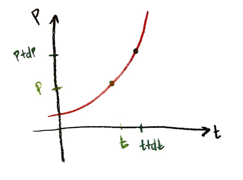
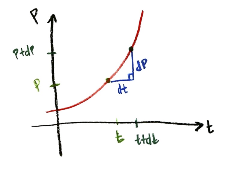
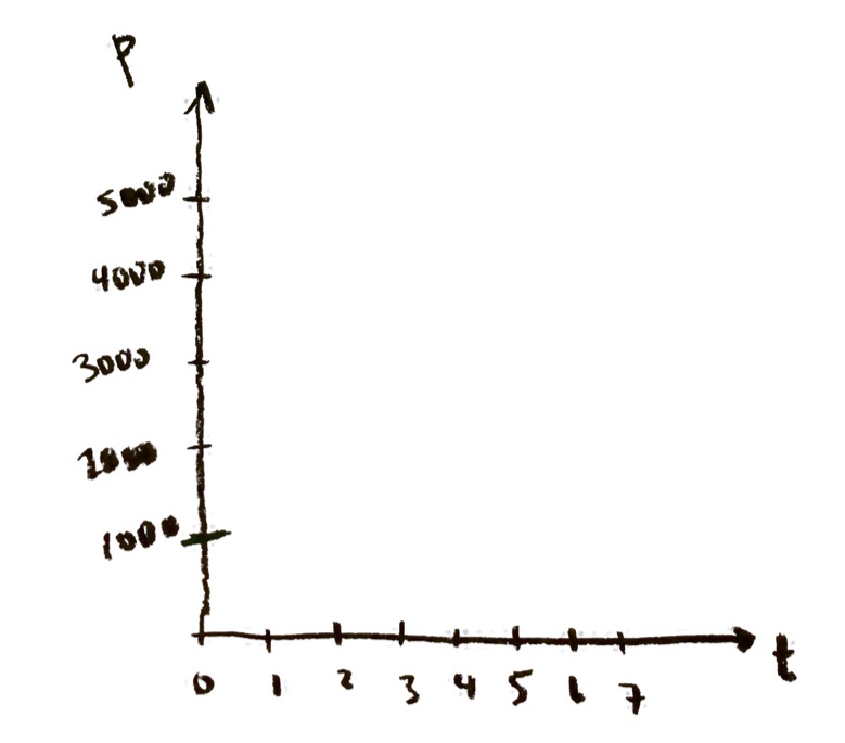
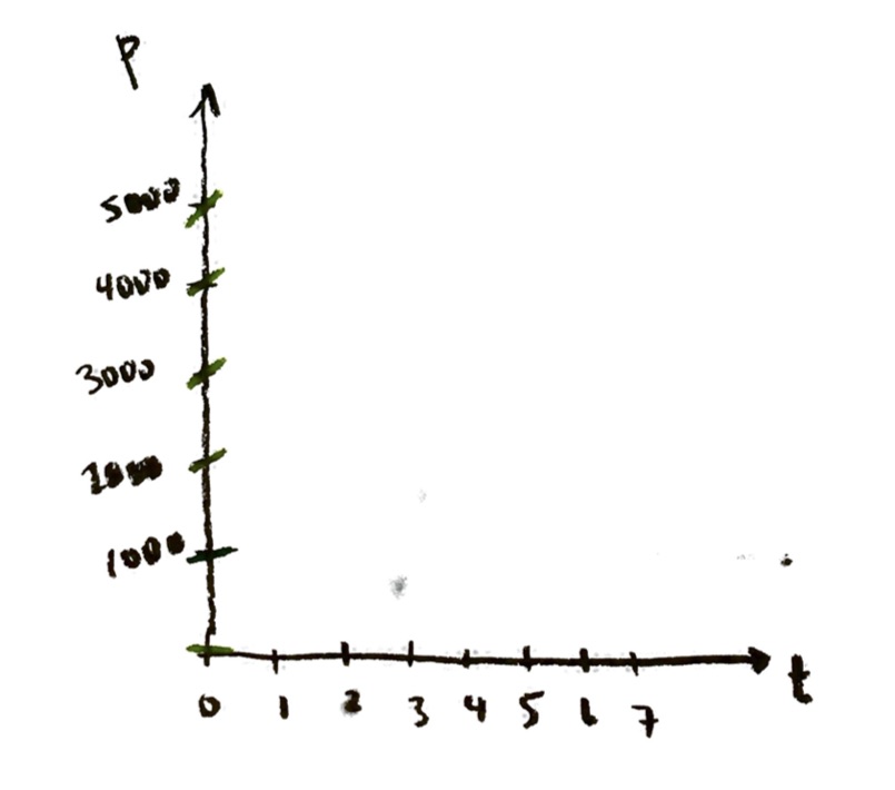
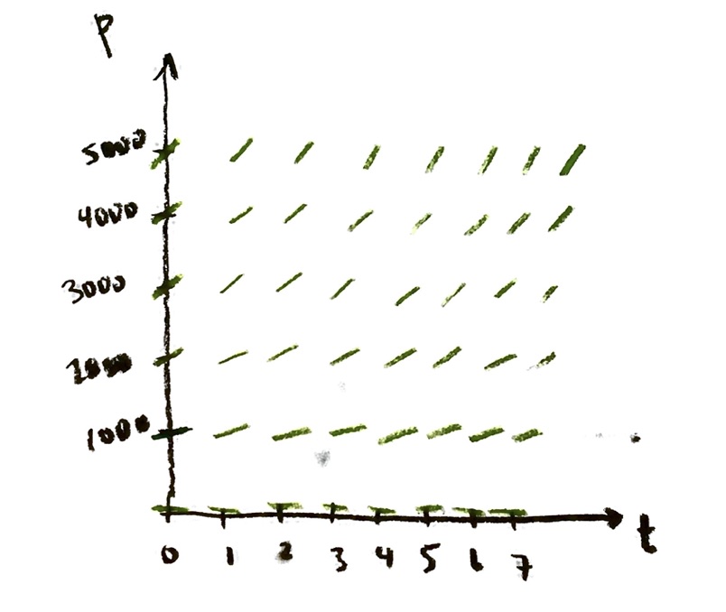
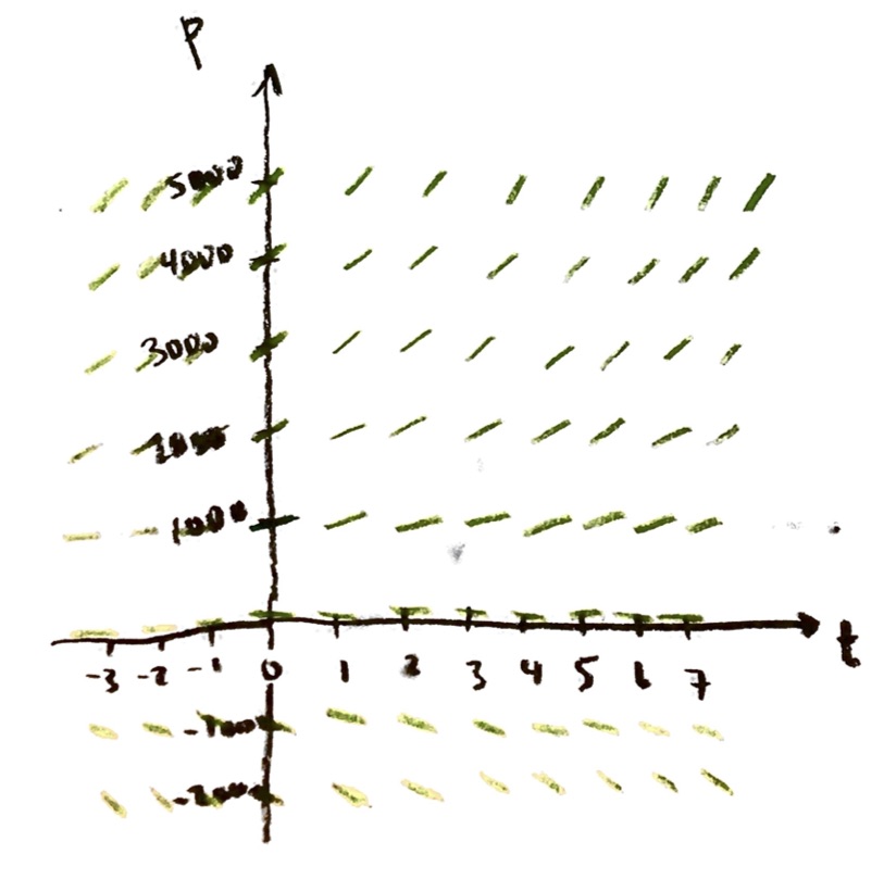
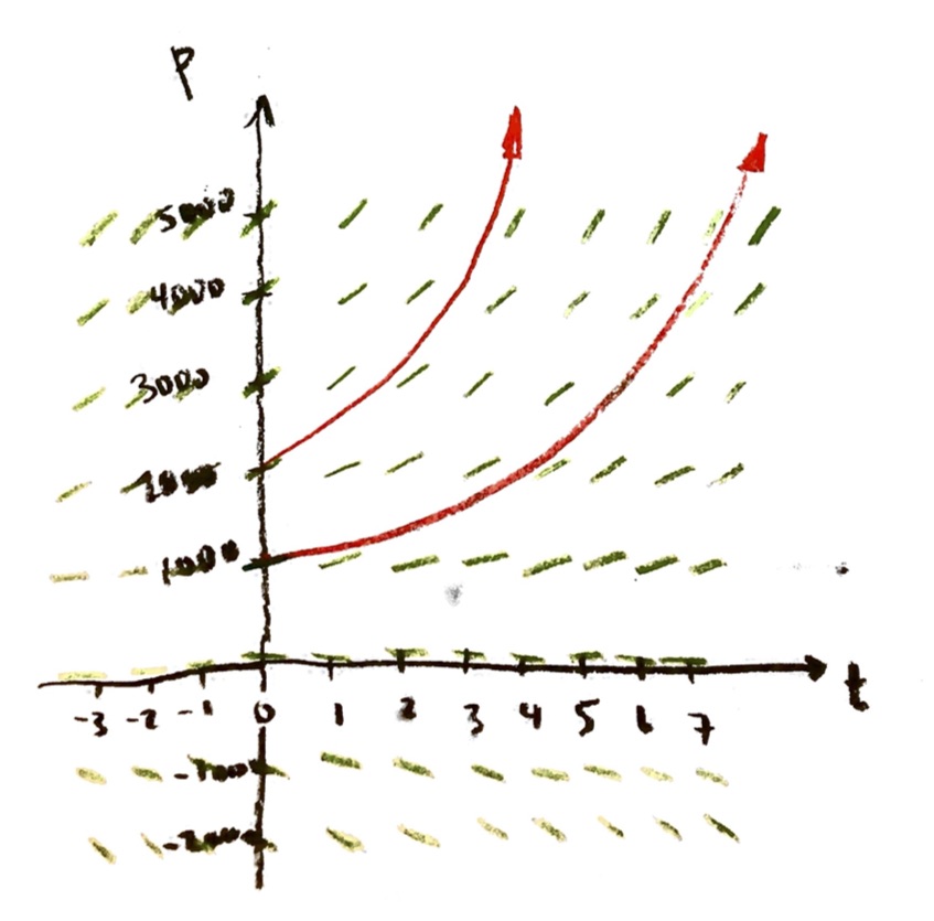
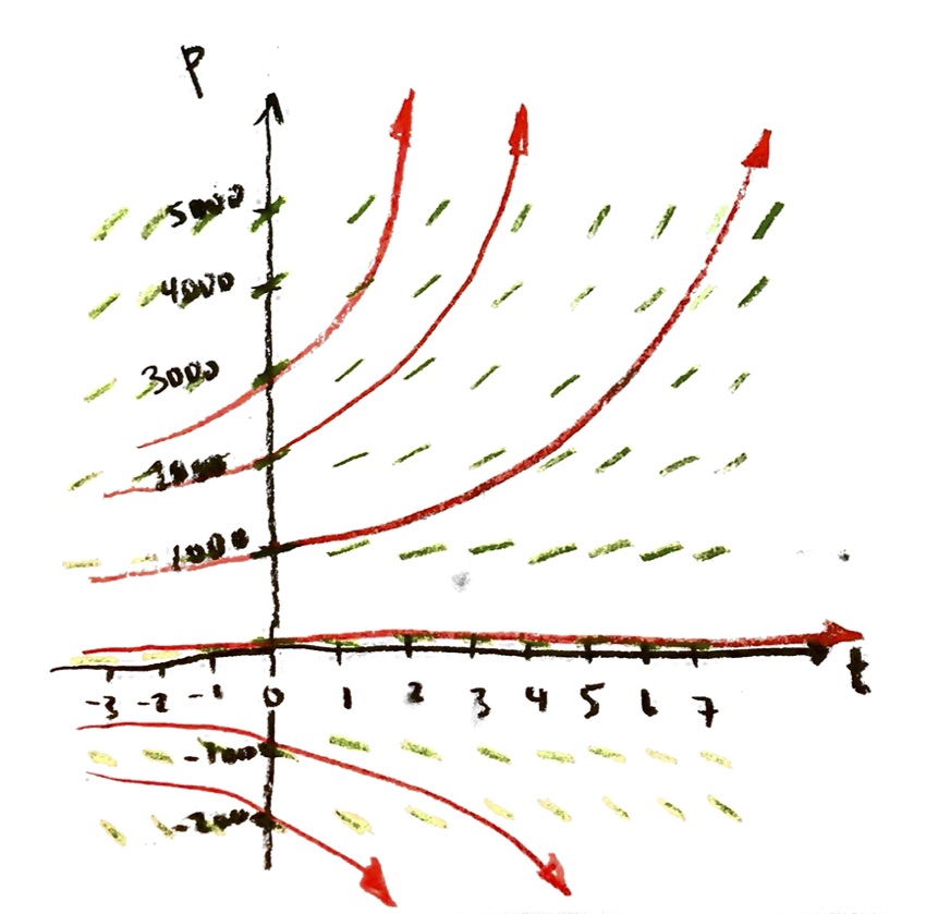
We have studied the “exponential growth” differential equation at some length now:

$\dfrac{\mathrm{d}P}{\mathrm{d}t}=rP$, where $r$ is a constant.

This models unrestricted continuous population growth. (It also models nuclear decay, and a number of other things.)

Since I don’t necessarily want to be modeling population with time, let’s switch to more generic variables y and x:

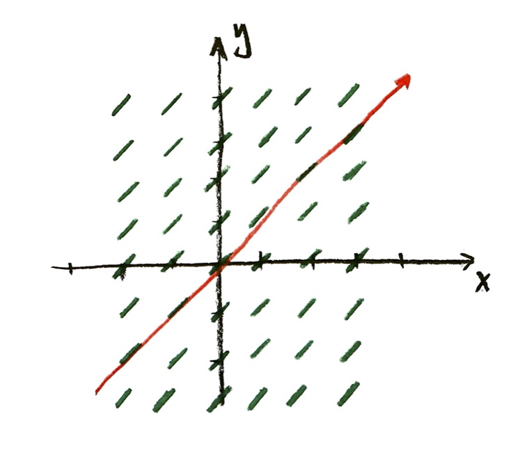
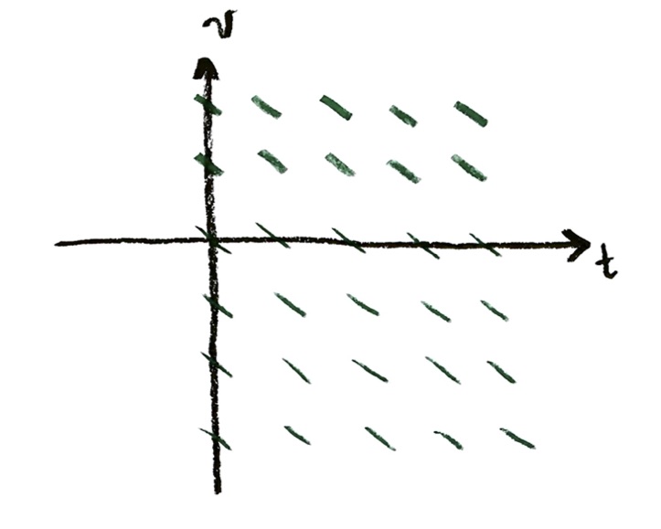
$\dfrac{\mathrm{d}y}{\mathrm{d}x}=ry$, where $r$ is a constant.

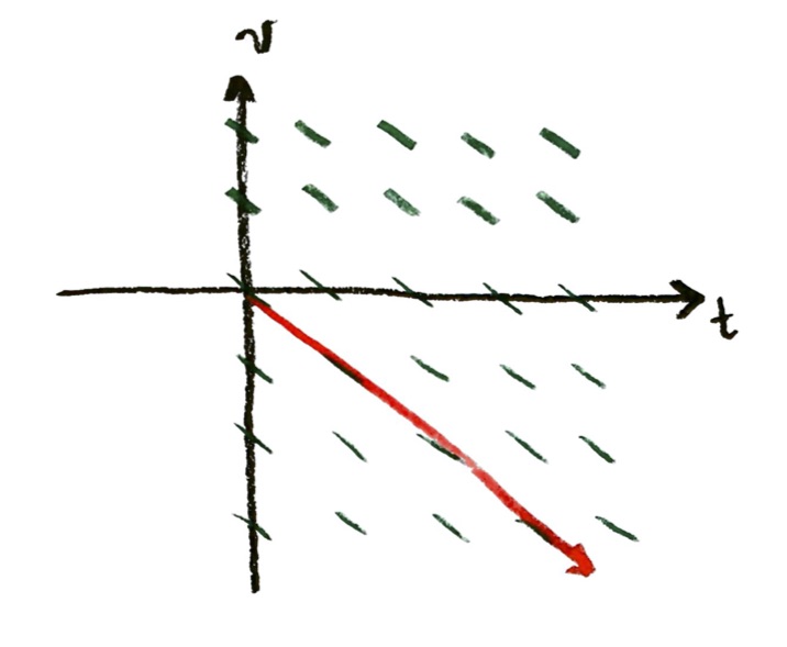
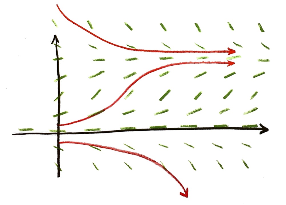
Taking r=1, we drew the slope field. Assuming that we start at y=1 when x=0, we found an equation for the solution curve:

$y=e^x$

where $e\doteq2.7182818284590452353602874713526624977572470936999595749669676277240766303535475945713821785251664274274663919320030599218174135\ldots$. The number $e$ is found by the formula

$e=\lim_{\Delta t\to 0}\left(1+\Delta t\right)^{\frac{1}{\Delta t}}$;

we gave an argument for why that was so in class. (In case you’re curious, here is the number e to one million decimal places!)

The equation $y=e^x$ is the solution (i.e. equation of the solution curve) for the problem

$\dfrac{\mathrm{d}y}{\mathrm{d}x}=y$, and y=1 when x=0.

Let’s elaborate and expand on this a bit.

power series for exponential function

In class, I described trying to solve the the differential equation

$\dfrac{\mathrm{d}y}{\mathrm{d}x}=y$, and y=1 when x=0,

by means of an “infinite polynomial”, or power series. I started off looking for a solution with y as a power of x, $y=x^n$. That can’t possibly work, because the differential equation says that the derivative of the function y with respect to x should equal the original function I started with! If $y=x^n$, then

$\dfrac{\mathrm{d}y}{\mathrm{d}x}=nx^{n-1}$,

and there is no way that $x^n$ and $n x^{n-1}$ can be equal functions. (Their numerical values could be equal for some particular values of x, certainly. But the differential equation is saying that the two formulas should be equal for all values of x—that is, that they should define the same solution curve—and that can’t possibly happen for $x^n$ and $n x^{n-1}$.)

I run into the same problem with any polynomial formula for $y$, because, for example, if $y=x^{10}+3x^5-x^3$, then the highest power of $x$ in the derivative of $y$ would be an $x^9$; therefore, the formula of the derivative cannot equal the formula of the original $y$.

But we wouldn’t run into this problem if $y$ was a “polynomial” that did not have a highest power!

So, I assume that the unknown function y of x I’m looking for can be written in the form

$y=a_0 + a_1x + a_2 x^2 + a_3 x^3 + a_4 x^4 + a_5 x^5 + a_6 x^6 + a_7 x^7 +\dotsb$,

where the $a_0$, $a_1$, $a_2$, . . . are some unknown numbers. Note that at this point, I do not know whether this is actually going to work! I have no particular reason to believe that the solution curve $y$ can be written this way. I’m just going to try it, and see if it works. I might run into a roadblock, like I did when I tried ordinary polynomial formulas; in that case, I’d have to back up and try something different. Or, it might work out.

(If it does work out, then I don’t have to worry if the path I took to get to the answer was kind of mysterious or illegal. The problem is to find a solution of the differential equation. If you can cook up an answer some crazy way, like seeing it in a dream, that’s fine: as long as you can show it satisfies the equation, it’s got to be correct!)

Alright: suppose the function y of x is given by this “infinite polynomial” (power series),

$y=a_0 + a_1x + a_2 x^2 + a_3 x^3 + a_4 x^4 + a_5 x^5 + a_6 x^6 + a_7 x^7 +\dotsb$,

and suppose that it satisfies the differential equation

$\dfrac{\mathrm{d}y}{\mathrm{d}x}=y$, and y=1 when x=0.

Let’s see if we can find the constants $a_0$, $a_1$, $a_2$, . . . based on these assumptions.

Problem: Power Series for $e^x$ (see below for answers!)
a. Use the initial condition, y=1 when x=0, to determine one of the constants.
b. Find the derivative of the power series formula representing the function $y$. (Your answer should be another infinite power series.)
c. Suppose that $\dfrac{\mathrm{d}y}{\mathrm{d}x}=y$. This should mean that two infinite power series are equal, as functions. That is, the numbers in front of each power of x should be the same in both formulas. Use this to give an infinite list of conditions on the $a_i$ constants.
d. Solve for all the $a_i$!
e. Put your answers back in the assumed series for y, to obtain a final formula for y.

Answers:

a. Setting y=1 and x=0 into the assumed formula for y, we end up with

$1=a_0+a_1(0)+a_2(0)+a_3(0)+\dotsb$

so we get $a_0=1$. We know one of the constants now!

b. Using what we did in Problem Sets 1 and 2, the derivative of

$y=a_0 + a_1x + a_2 x^2 + a_3 x^3 + a_4 x^4 + a_5 x^5 + a_6 x^6 + a_7 x^7 +\dotsb$,

is

$\dfrac{\mathrm{d}y}{\mathrm{d}x}=a_1 + 2a_2 x + 3a_3 x^2 + 4a_4 x^3 + 5a_5 x^4 + 6a_6 x^5 + 7a_7 x^6 +\dotsb$.

c. I am assuming that the only way these two functions, $y$ and $\dfrac{\mathrm{d}y}{\mathrm{d}x}$, can be equal, is if they have exactly the same formula; that is, if the number in front of $x^n$ is the same in each formula for every power $n$. (I’m making an assumption here; if we were doing things more carefully, I’d need to prove that is actually true.)

This only works if we have:

$a_1=a_0$, $2a_2=a_1$, $3a_3=a_2$, $4a_4=a_3$, $5a_5=a_4$, . . .

d. Let me write these slightly differently:

$a_1=a_0$, $a_2=\frac{1}{2}a_1$, $a_3=\frac{1}{3}a_2$, $a_4=\frac{1}{4}a_3$, $a_5=\frac{1}{5}a_4$, . . .

But we know $a_0=1$! So we can solve these “recursively”:

$a_1=a_0=1$

$a_2=\frac{1}{2}a_1=\frac{1}{2}(1)=\frac{1}{2}$

$a_3=\frac{1}{3}a_2=\frac{1}{3}\frac{1}{2}=\frac{1}{3\cdot 2}$

(That dot in the last denominator is a “times”. I’m writing $a_3$ as $\frac{1}{3\cdot 2}$ rather than $\frac{1}{6}$, because I want to be able to see the pattern more easily. But it is just $a_3=\frac{1}{6}$.)

$a_4=\frac{1}{4}a_3=\frac{1}{4}\frac{1}{3}\frac{1}{2}=\frac{1}{4\cdot 3\cdot 2}$

$a_5=\frac{1}{5}a_4=\frac{1}{5}\frac{1}{4}\frac{1}{3}\frac{1}{2}=\frac{1}{5\cdot 4\cdot 3\cdot 2}$

Now you can see the pattern:

$a_n=\frac{1}{n\cdot (n-1)\cdot \dotsb \cdot 4\cdot 3\cdot 2\cdot 1}$

(I put the “times 1” at the end just to make the pattern more consistent looking. Of course it doesn’t change anything.)

Since this pattern happens a lot in math, we have a name (“factorial”) and a symbol for it: for any whole positive number n, we define

$n!=n\cdot (n-1)\cdot \dotsb \cdot 4\cdot 3\cdot 2\cdot 1$.

e. Putting these back into the formula for y, we get

$y=1+x+\frac{1}{2!}x^2+ \frac{1}{3!}x^3+\frac{1}{4!}x^4+\frac{1}{5!}x^5+\dotsb$

Since we already know that $y=e^x$, we get

$e^x=1+x+\frac{1}{2!}x^2+ \frac{1}{3!}x^3+\frac{1}{4!}x^4+\frac{1}{5!}x^5+\dotsb$

Checking the solution

Remember that I assumed that y could be written as

$y=a_0 + a_1x + a_2 x^2 + a_3 x^3 + a_4 x^4 + a_5 x^5 + a_6 x^6 + a_7 x^7 +\dotsb$

for some constants $a_0$, $a_1$, $a_2$, . . . And, pushing through with a spirit of hope, we found that if that is true, then in fact

$y=1+x+\frac{1}{2!}x^2+ \frac{1}{3!}x^3+\frac{1}{4!}x^4+\frac{1}{5!}x^5+\dotsb$

This should supposedly be a solution to the problem

$\dfrac{\mathrm{d}y}{\mathrm{d}x}=y$, and y=1 when x=0.

But is it? The path I took to get here is a little suspicious. Let’s try to check this.

Problem: Checking power series solution for exponential function
a. With y given by the formula above, check that y=1 when x=0. (This shouldn’t be hard!)
b. Find the derivative of y with the formula given above. Does taking the derivative give you back the original formula, as it was supposed to?

There is another thing to worry about. Remember when we found an infinite series for the function $1/(1+x)$, which came out

$\dfrac{1}{1+x}=1-x+x^2-x^3+x^4-x^5+x^6-x^7+\dotsb$?

If you recall, this formula worked out great if the x value was small enough, specifically $-1<x\leq 1$. But it made no sense for larger values.

Something similar can happen with this technique for solving a differential equation: we can get a formula which is correct, but only in a limited range.

Happily, as it turns out, our power series for $y=e^x$ actually gives correct answers for all values of $x$. (If you take a more advanced course, we would prove that.)

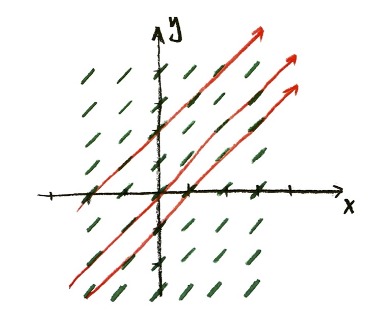
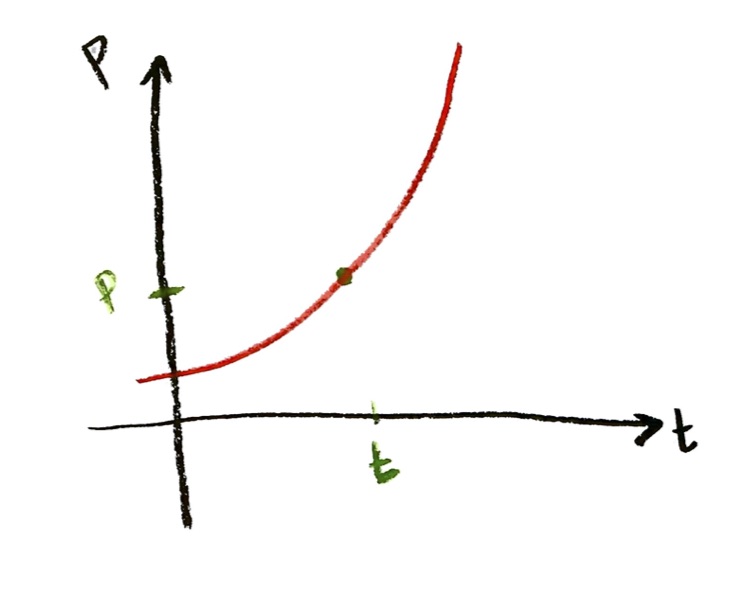
Solution with different initial conditions

Suppose that instead of starting with y=1 when x=0, we started with some other value $y=y_0$ at x=0. (In the population model, the value of $y_0=P_0$ would correspond to our starting population at time t=0.)

There are two ways we could find the formula for the solution. First way: we could go back to the same procedure we did above, just with a different starting point. It will be good practice to work this out yourself:

Problem: Exponential differential equation with different initial condition
As before, assume that we are trying to solve $\dfrac{\mathrm{d}y}{\mathrm{d}x}=y$, but now we are assuming $y=y_0$ when $x=0$. As before, assume that $y$ can be written in the form $y=a_0 + a_1x + a_2 x^2 + a_3 x^3 + a_4 x^4 + a_5 x^5 + a_6 x^6 + a_7 x^7 +\dotsb$.
a. Use the initial condition to determine the $a_0$. (“Determine” means it will be in terms of $y_0$.)
b. Repeat the process that you did before, to get $a_1$ in terms of $a_0$, to get $a_2$ in terms of $a_1$, etc etc. It should all work out very similarly, except for a $y_0$ in each of your formulas.
c. Put the answers all back into $y=a_0 + a_1x + a_2 x^2 + a_3 x^3 + a_4 x^4 + a_5 x^5 + a_6 x^6 + a_7 x^7 +\dotsb$, to get the formula for y. (It will involve $y_0$.)
d. If you haven’t already, try to simplify y. (Hint: You should be able to write it so there is only one $y_0$ in your entire formula.)
e. Compare to the answer you got before, when $y_0=1$. Can you write this solution in terms of the earlier solution?

The answer to the last part should be the following: you will end up with

$y=y_0 e^x$.

This solves the differential equation $\dfrac{\mathrm{d}y}{\mathrm{d}x}=y$, with the initial condition $y=y_0$ when $x=0$.

There is a second way: we can make a change of variable. This is what Thompson calls a “useful dodge”. Here’s how it works. Suppose we want to solve the differential equation

$\dfrac{\mathrm{d}y}{\mathrm{d}x}=y$, with initial condition $y=y_0$ when $x=0$.

I introduce a new variable $u$, which is defined by $y=y_0 u$. Since $y_0$ is a constant, if I vary u a little bit to $u+\,\mathrm{d} u$, then the corresponding $\mathrm{d} y$ is given as follows:

$y+\mathrm{d} y = y_0\left(u+\mathrm{d}u\right)$
$y+\mathrm{d} y = y_0 u+y_0\mathrm{d}u$
$\mathrm{d} y = y_0\mathrm{d}u$

So, dividing by $\mathrm{d}x$ on both sides, we get

$\dfrac{\mathrm{d} y}{\mathrm{d} x}=y_0\dfrac{\mathrm{d}u}{\mathrm{d} x}$.

(We could have also got the same result by the derivative rules.)

Substituting this, and $y=y_0 u$, into the differential equation $\dfrac{\mathrm{d}y}{\mathrm{d}x}=y$, we get the differential equation

$y_0\dfrac{\mathrm{d} u}{\mathrm{d} x}= y_0 u$,

from which I can cancel the $y_0$ on both sides, and get

$\dfrac{\mathrm{d} u}{\mathrm{d} x}= u$.

That’s exactly the same differential equation as I started with for y! What is the initial condition? Well, when $x=0$, we have $y=y_0$. Then, putting this into $y=y_0 u$, we get $y_0=y_0 u$, so $u=1$. That is, the initial condition is, when $x=0$, we have $u=1$. So our problem is:

$\dfrac{\mathrm{d} u}{\mathrm{d} x}= u$, and $u=1$ when $x=0$.

That’s exactly the problem we started with!! So it has the same solution:

$u=e^x$.

I want to go back to the original variable, so I’ll multiply both sides by $y_0$:

$y_0 u = y_0 e^x$.

Using $y=y_0 u$, we get:

$y=y_0 e^x$.

That solves the problem

$\dfrac{\mathrm{d}y}{\mathrm{d}x}=y$, and y=y_0 when x=0,

and it agrees with the solution we found the first way.

Problem: Checking the solution again
Check this directly. That is, start with $y=y_0e^x$. Knowing that the derivative of $e^x$ is $e^x$, use this to find the derivative of $y=y_0e^x$. Check that it satisfies the differential equation $\dfrac{\mathrm{d}y}{\mathrm{d}x}=y$. Also, substitute in $x=0$ to check that then $y=y_0$.

Solution with a different rate

We had started with the exponential growth differential equation,

$\dfrac{\mathrm{d}P}{\mathrm{d}t}=rP$, and $P=P_0$ when $t=0$.

where $r$ is some constant. The last little while, I’ve been assuming $r=1$ to make things simple. But now it’s time to put the $r$ back in.

(I am going to change from $y$ and $x$ back to $P$ and $t$ for these problems, just for variety. It doesn’t really change anything.)

Again, there are two ways to proceed! First way, do the same procedure that we started with from the beginning, with the infinite series:

Problem: Exponential growth with rate r, by infinite series
Suppose we want to solve $\dfrac{\mathrm{d}P}{\mathrm{d}t}=rP$, and $P=P_0$ when $t=0$. Start by assuming that
$P=a_0+a_1 t + a_2 t^2 + a_3 t^3 + a_4 t^4+\dotsb$.
a. Find the value of $a_0$, in terms of $P_0$.
b. Find the derivative of the power series representing $P$.
c. Find $rP$, where you will substitute in the power series for $P$, and multiply all the terms through by $r$.
d. Setting $\frac{\mathrm{d}P}{\mathrm{d}t}=rP$, you have two power series that are supposed to be equal. Use this to get conditions on the $a_1$, $a_2$, $a_3$, . . .
e. Solve the conditions to find the values of the $a_1$, $a_2$, $a_3$, . . .
f. Put the answer back in the power series, to find the formula for P. Simplify it as much as you can.

I won’t give the answers right away, but you will be able to check your answers against the second method.

The second method is to make a change of variable (the “useful dodge”):

Problem: Exponential growth with rate r, by change of variable (see below for answers!)
Introduce a new variable $s$, defined by $s=rt$.
a. Find the relationship between $\mathrm{d} s$ and $\mathrm{d}t$. (Remember that $r$ is a constant.)
b. Substitute this into the differential equation $\frac{\mathrm{d}P}{\mathrm{d}t}=rP$, to get a differential equation for $P$ as a function of $s$ (that is, eliminate the variable t).
c. Recognize this as a differential equation you can solve! Check the initial condition, and write out the answer for P as a function of s.
d. Make a substitution to write P as a function of t, which is the final answer.

Answers:

a. $\mathrm{d} s = r\,\mathrm{d} t$.

b. There’s different ways to do the algebra. I find it convenient to rewrite the differential equation as

$\mathrm{d}P=rP\,\mathrm{d}t$.

Then I can identify $r\,\mathrm{d} t$ as $\mathrm{d} s$, so

$\mathrm{d}P=P\,\mathrm{d}s$,

or

$\dfrac{\mathrm{d}P}{\mathrm{d}s}=P$.

c. This is just the original differential equation! And the initial condition is the same, too, because when $s=0$, we have $t=0$, so $P=P_0$ when $s=0$. So the solution is

$P=P_0 e^s$,

as in the previous section.

d. Now, we can put back $s=rt$, to find

$P=P_0 e^{rt}$

as the solution of

$\dfrac{\mathrm{d}P}{\mathrm{d}t}=rP$, and $P=P_0$ when $t=0$.

Nice!

You can use this to check your answer by the first method. For the first method, you should have gotten

$P=P_0\left(1+rt+\frac{1}{2!}r^2t^2+\frac{1}{3!}r^3t^3+\frac{1}{4!}r^4t^4+\dotsb\right)$

You can rewrite this as

$P=P_0\left(1+(rt)+\frac{1}{2!}(rt)^2+\frac{1}{3!}(rt)^3+\frac{1}{4!}(rt)^4+\dotsb\right)$

and that is the same as substituting (rt) in everywhere for the original exponential series we got. That is,

$P=P_0e^{rt}$,

which agrees with the second method.

Trigonometric functions

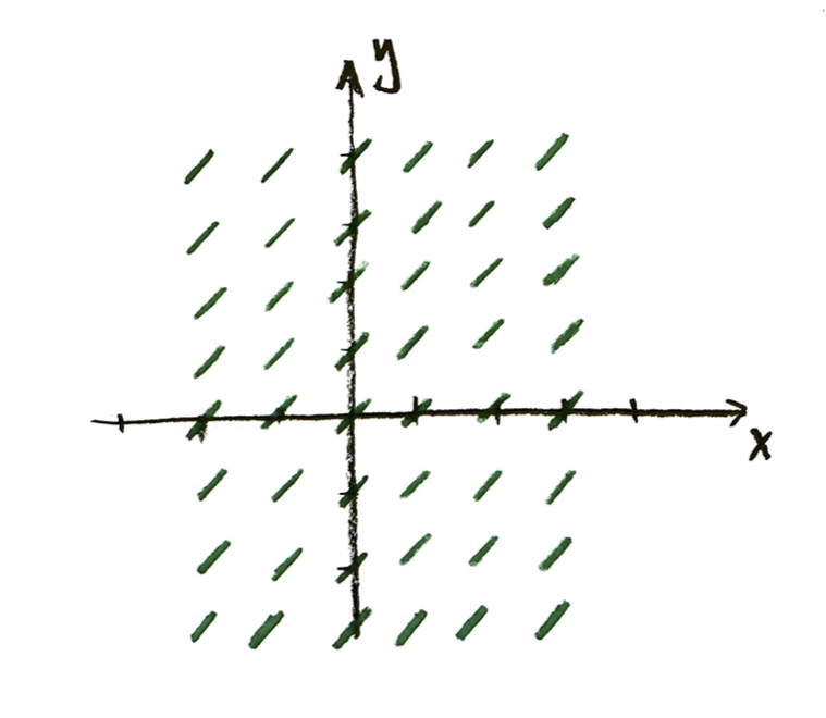
Now, I want to refer back to what we did on trigonometric functions, in Problem Set #6, Problems #5 and 6. First, a quick reminder of the setup. I was starting with a circle of radius 1, whose center was at the origin (0,0) of an x-y coordinate system. I was starting at the point (1,0) on the circle, and then traveling a distance s counter-clockwise along the edge of the circle.

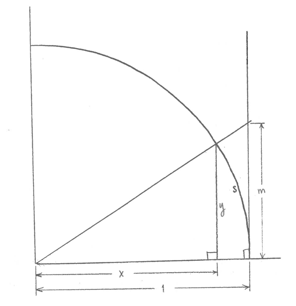
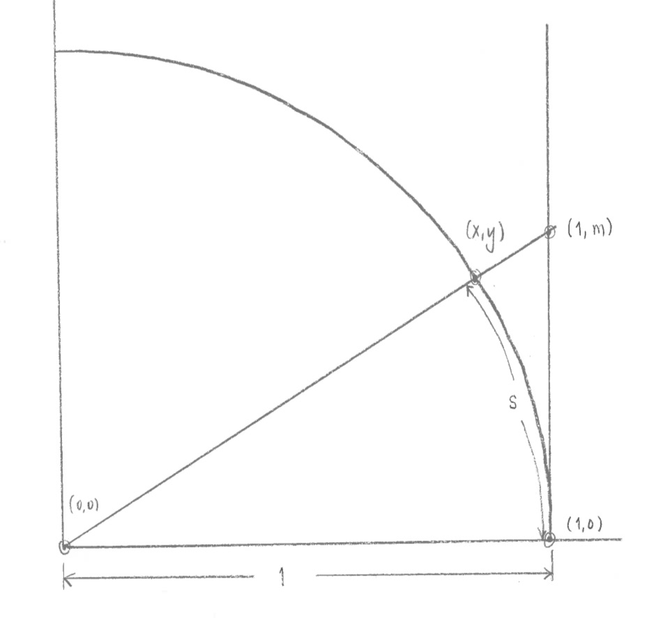
After traveling a distance s counter-clockwise along the edge of the circle, starting at (1,0), I end up at a point (x,y). I wanted to find formulas for x and y in terms of s. Or similarly, to find formulas for s in terms of x or in terms of y.

Now, there is a trig answer:

$x=\cos s$ and $y=\sin s$.

You could either prove these facts, assuming the definitions you learned in high school for cosine and sine (based on right triangles), and using the diagram above. Or, another way of looking at things is to define the functions cosine and sine by this diagram, so that the two formulas above are true by definition. This is the way I will think of it. (Then the high school definitions of cosine and sine follow from this definition.)

Note that this doesn’t totally answer my question: I do not have any way of calculating x or y if I know s. Saying that $x=\cos s$ is just a way of naming the relationship. If I have a calculator, and I know s, I can find x; but how is the calculator doing that??

In what follows, I’m going to look for an actual formula for x and y in terms of s, which will actually let me find the x and y numerically if I know the s. (In another way of speaking, it will give us an actual formula for the cosine and sine functions.)

Remember also that I increased the s slightly to $s+\,\mathrm{d}s$, which changed the point $(x,y)$ to the point $(x+\,\mathrm{d}x,y+\,\mathrm{d}y)$. In Problem Set #6, I asked you to try to figure out $\mathrm{d}x$ and $\mathrm{d}y$ in terms of $\mathrm{d}s$. Here were the answers:

$\mathrm{d} x = -y \,\mathrm{d}s$
$\mathrm{d} y = x \,\mathrm{d}s$.

That translates to two differential equations:

$\dfrac{\mathrm{d} x}{\mathrm{d}s} = -y $
$\dfrac{\mathrm{d} y}{\mathrm{d}s} = x $.

There are two unknown functions, x and y, which each depend on the variable s. Their differential equations are interlocked: the derivative of the unknown function y equals the unknown function x; the derivative of the unknown function x equals the negative of the unknown function y.

We also have initial conditions: looking at the diagram, if $s=0$, then we are at the point $(1,0)$, which means $x=1$ and $y=0$ when $s=0$.

We can attempt to solve these differential equations by the same method as before, with the infinite power series. There are now two unknown power series:

$x=a_0 + a_1 s + a_2 s^2 + a_3s^3 + a_4 s^4 + a_5s^5 + a_6 s^6 + \dotsb$
$y=b_0 + b_1 s + b_2 s^2 + b_3s^3 + b_4 s^4 + b_5s^5 + b_6 s^6 + \dotsb$

Here, the $a_0$, $a_1$, $a_2$ . . . and the $b_0$, $b_1$, $b_2$ . . . are all unknown constants. (These are different from the $a_0$, $a_1$, $a_2$ from before for the exponential function.)

We can use initial conditions and differential equations to solve for all these unknown constants:

Problem: Power Series for sine and cosine
a. Use the initial conditions to find the values of $a_0$ and $b_0$.
b. Find the derivative of the power series for $x$, and of the power series for $y$.
c. Find the power series for $-y$. (Just multiply through the minus sign times every coefficient of the power series for $y$.)
d. Now, use the equalities $\frac{\mathrm{d} x}{\mathrm{d}s} = -y $ and $\frac{\mathrm{d} y}{\mathrm{d}s} = x $ to say that two pairs of infinite power series should be equal. Use that to get two series of conditions that relate the $a_1$, $a_2$, $a_3$ . . . and the $b_1$, $b_2$, $b_3$, . . .
e. Solve these equations, to find the values of all the $a_1$, $a_2$, $a_3$ . . . and the $b_1$, $b_2$, $b_3$, . . .
f. Put the values of the $a_1$, $a_2$, $a_3$ . . . and the $b_1$, $b_2$, $b_3$, . . . back into the power series for x and y, to get formulas for x and y in terms of s.

Now that we have the solutions, this gives us an infinite power series for $x= \cos s$ and for $y=\sin s$. Once you have a tentative answer, you can check it:

Problem: Checking solutions for power series for sine and cosine
Take your power series for x, and take its derivative. It should come out to be the same as the negative of the power series for y. Does it? If not, you might need to simplify; or you might need to correct an error from the previous problem. Similarly, take your power series for y, and take its derivative; it should come out to be the same as your power series for x.

I don’t want to put the answers here, to give you a chance to work them out. However, if you look up “cosine power series”, you can find the answer.

It’s also interesting to check these answers graphically:

Problem: Graphing the power series for sine and cosine
Use Desmos to graph the function $y=\cos x$. (To use the grapher, we have to change our variable s to x, and x to y, which is maybe a little confusing!) Now, on the same axes, graph $y=1-(1/2)x^2$, which should be the first two terms of your power series for cosine (again, switching the variable s to x). There should be a nice fit near x=0 (s=0)! This is the “best fit parabola” to the function cosine at s=0. Now, graph the functions you get when you add in more and more terms of the power series. If everything is right, you should see these polynomials fitting more and more closely the cosine function.

Oscillations

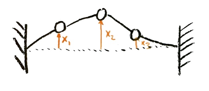
I won’t quite get to the Kepler problem in this problem set, although I’ll try to show how to solve it in a final optional lecture after this one. However, I can show you how these ideas come up in physics problems, by using a simpler physics problem.

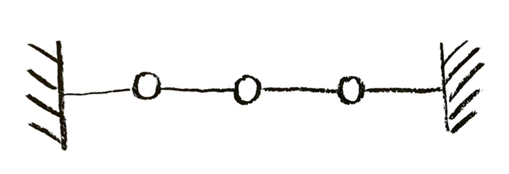
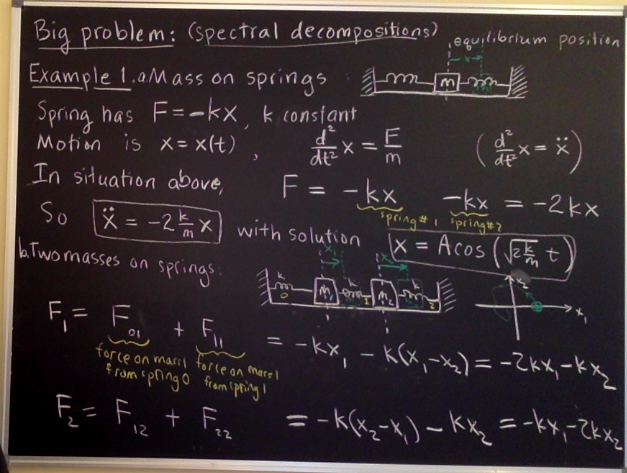
Let’s say we have a mass on a spring. I assume that the mass can only move in one direction, let’s call it the x-axis. I set up my coordinate so that the spring is at rest (not stretched or squeezed) when x=0. Then x is the displacement from rest. If $x>0$, the spring is stretched, and the mass experiences a force in the negative direction; if $x<0$, the spring is squeezed, and the mass experiences a force in the positive direction. In either case, the force is pushing the mass back towards x=0; such a force is called a restoring force, and x=0 is called a stable equilibrium.

The simplest model is to assume that the restoring force is simply proportional to the displacement from equilibrium:

$F=-kx$,

where $x$ is the displacement from equilibrium, and $k$ is some constant. Nearly any force approximately obeys this assumption for small enough displacements. So we can use it for a mass on a spring, but also for a swinging pendulum, or a swaying bridge: nearly any situation where there is a stable equilibrium and a restoring force, and where the displacements are not too large.

Using Newton’s law,

$a=\dfrac{F}{m}$,

we find that

$a=-\dfrac{k}{m} x$.

The acceleration, by definition, is the derivative of the velocity with respect to time; and the velocity, by definition, is the derivative of the displacement with respect to time. We have two unknown functions of time $t$, the position $x$ and velocity $v$, and we get two interlocked differential equations for those unknown functions:

$\dfrac{\mathrm{d}v}{\mathrm{d} t} = -\dfrac{k}{m} x$
$\dfrac{\mathrm{d}x}{\mathrm{d} t} = v$

This is suspiciously similar to our situation with the cosine and sine functions!! That is not a coincidence.

As before, we could take two strategies: we could start over with the unknown power series, and solve as before. We would get very similar answers to what we got for cosine and sine, with some $\frac{k}{m}$ factors thrown in. Or, second strategy, we could change variables. I will just outline the second strategy here.

Problem: Solving harmonic oscillator (partial answers below)
a. To start off with, let’s suppose that $\frac{k}{m}=1$. Let’s also suppose that the initial condition is $x=1$, and $v=0$, when $t=0$. In this case, compare to the differential equations we got before for the unit circle, for x and y in terms of s. They should be very similar! Use this similarity to write the position x and velocity v as functions of t. The functions should involve cosines and/or sines.
b. Does your answer make physically?
c. Now, if $\frac{k}{m}\neq 1$, we can try the change of variables trick. There’s something a little sneaky this time: I’m going to make a new variable s to replace t, by $s=\sqrt{\frac{k}{m}}t$, and I’m going to make a new variable w to replace v, by $v=\sqrt{\frac{k}{m}}w$. I’m going to leave x as just x. (If I had more time, I could explain where I got these!!) Use these equations to find the relation of $\mathrm{d}s$ and $\mathrm{d}t$, and also the relation of $\mathrm{d}v$ and $\mathrm{d}w$. Put the relations into the differential equations. You should find, once everything is simplified, that you get the equations
$\dfrac{\mathrm{d}w}{\mathrm{d} s} = – x$
$\dfrac{\mathrm{d}x}{\mathrm{d} s} = w$
d. Assuming we again start with $x=1$ and $v=0$ when $t=0$, use that to give initial conditions for $x$ and $w$, when $s=0$. Then give the solutions to the differential equations for x and w, as functions of s.
e. Finally, substitute back in, to find the position x and velocity v as functions of time t.

Something that is remarkable here is that the differential equation for oscillation is very physically natural. If we try to solve this differential equation, we get the power series for cosine and for sine (for the position and velocity). So, even if we never cared about triangles at all, the cosine and sine functions would be forced on us by physics and differential equations. In fact, this is the more calculus-style way of defining cosine and sine: we define them to be the solution of the differential equations I wrote earlier. Then we would use that to prove that they in fact give the x and y coordinates of that point on the circle, and use that to finally say they happen to equal opposite/hypotenuse and adjacent/hypotenuse.

And finally, some magic

I want to finish with a formula that I think is kind of magical. It is not just a nice mathematical formula though; it is very important in engineering and physics, for example. It will give a simpler way of solving the oscillation problem we just did, and it will allow for oscillations with damping (though we won’t have time to get to that: take ordinary differential equations next term!).

First, I need to remind you / tell you about complex numbers. You may recall that a negative number cannot have a square root. There cannot be any normal number x such that

x times x equals -1,

because (positive)*(positive)=positive, and (negative)*(negative)=positive. So $\sqrt{-1}$ has no meaning in ordinary (“real”) numbers. However, as early as the 1400s, people identified instances where having a square root for negative numbers would be mathematically convenient. It turns out that many things in mathematics (and physics) work out much more nicely if you allow for negative numbers to have square roots. This requires us to expand our concept of “number” to “complex numbers” (which contain the real numbers). Complex numbers turn out to be inextricably part of quantum mechanics, which makes them part of reality! They are not just a convenient mathematical invention.

We simply declare the existence of a new number, which we call $i$, which has the property that

$i^2=-1$.

This means $\sqrt{-1}=\pm i$. Similarly, $\sqrt{-4}=\pm 2 i$. (You can check these claims by squaring $i$ and $-i$, and seeing you get -1 in both cases; or squaring $2i$ and $-2i$, and seeing that you get -4 in both cases.)

A complex number is any number I can make by combining real numbers with any expressions involving $i$. It turns out that the parts involving $i$ can always be greatly simplified; in fact, any algebraic mess you can make with real numbers and $i$s can always be boiled down to $x+iy$, for some real numbers $x$ and $y$.

As an illustration, try the following:

Problem: Powers of $i$
a. Simplify $i^3$. (Remember that $i^3=i\cdot i\cdot i$.)
b. Simplify $i^4$. (Hint: this one should come out to be very simple!!)
c. Simplify $i^5$, $i^6$, $i^7$, $i^8$, $i^9$.
d. What’s the pattern?
e. Simplify $i^{403}$.

If this was specifically about complex numbers, I would go on to tell you how to simplify things like $1/(1+i)$ or $\sqrt{i}$. But what you did in the problem is enough to tell you the magical thing I want to tell you.

Here’s what I want you to try: to simplify the function $y=e^{ix}$, where $i^2=-1$ as above.

Problem: The function $y=e^{ix}$
a. Recall the power series for $y=e^x$ that you found, at the beginning of this problem set. In that series, substitute in $ix$ every place there is an $x$, to obtain the series for $y=e^{ix}$. (Be sure to put the $ix$ in as one unit in place of the $x$, with parentheses as needed. For example, if there is an $x^2$ in the power series for $y=e^x$, replace that $x^2$ with $(ix)^2$, so that that $i$ will get squared as well.
b. Replace $(ix)^2=i^2x^2$, $(ix)^3=i^3x^3$, etc.
c. Now, use the simplifications you made for powers of $i$.
d. You will find that half the terms have an $i$, and half do not. Collect all the terms without any $i$ in them all first, and then collect all the terms that do have an $i$ in them afterwards. If everything is correct, you should be able to factor out a common “$i$” out of all the latter half of the terms: do so.
e. Now, you should have one power series without any $i$, plus $i$ times a second power series. You should recognize each of those power series from a previous question! Use what those power series represent, to write $e^{ix}$ in terms of other known functions.

I don’t want to write the answer here, because I don’t want to spoil the punch line. But if you are stuck, and want to see what answer I am aiming for, or you want to check your answer, google the term “Euler’s formula” and you’ll see what I’m talking about. (There are actually a bunch of different things called “Euler’s formula”—he did a lot of formulas—but the first hit should be the formula I’m talking about here.)

Conclusion

There is so much more I want to tell you about! We’ve just started on all the cool things there are in calculus. But this is a good stopping point for this term: I think, if you’re caught up till now, then you should hopefully be able to do most of this problem set before the end, and be able to see a nice wrapping-up point.

If I have the time and energy, I will post an “epilogue” problem set, in which I will try to show you some of the cool things I have left out. In particular, I had promised you a derivation of Kepler’s laws. We’re nearly there (so close!), but I don’t want to overwhelm you; so I’ll put those in the optional “epilogue” (which I hope I’ll have the energy to write!). Either way, I’ll be giving you some references for further reading.

Hi everyone!

This follows the lecture on Differential Equations.

This lecture combines two things: I will give some more examples of setting up a differential equation model, and graphing the slope field.

I will also ask you some problems, which I would like you to submit, so I’m also going to call this lecture “Problem Set #8”. Please submit these problems, over slack as usual. You can submit them one at a time. Please indicate in the message the problem set and the problem name, e.g. “Problem Set 8: Numerically approximating the solution of a differential equation”.

I’m mixing the examples together with the problems so that I can explain the problems before getting you to do them, with extra examples as necessary.

Problem: Approximately numerically solving a differential equation

I’d like to start by getting you to do an example like in the previous lecture. In that lecture, I started with the difference equation

$\Delta P = (0.10) P \Delta t$,

describing population growth, at a 10% per time period rate.

At first, I took $\Delta t=1$: that meant that 10% was added to the population discretely, once every time period, and I tabulated it. That is a good population model if the animals have a definite breeding season, for example.

But then, I imagined that the reproduction was happening continuously. In this case, the population does NOT grow by 10% in one hour. Even though that is the continuous rate, after an hour, we will actually have more than 10% added!

That’s because, in that first hour, individuals were being added, and they contribute to the growth. For example, I started looking at half time periods, $\Delta t=0.5$. In the first half time period, the population would increase by 5%; those extra 5% would then reproduce in the next half hour.

But that’s not really good enough, if the growth is continuous: in that first half hour, individuals are added as well. So I split it into quarter time periods $\Delta t=0.25$, tenths of time periods $\Delta t=0.1$, . . . and tabulated those. (Look at the previous lecture to see what I’m talking about!)

Continuous growth would be the limiting values of that table, as I take the $\Delta t$ smaller and smaller. The limiting case would be a solution of the differential equation

$\mathrm{d}P = (0.10) P \,\mathrm{d}t$

or

$\dfrac{\mathrm{d}P}{\mathrm{d}t} = (0.10) P$

OK, I’d like you to try this yourself:

Problem: Numerically approximating the solution of a differential equation
Suppose we want to solve the differential equation

$\mathrm{d}P = P \,\mathrm{d}t$.

(I have replaced the rate $r=0.10$ in the example I did, with $r=1$ instead. So the organisms are reproducing at a continuous rate of 100% per time period.) Suppose that the initial population is $P=1000$ at time $t=0$. I want you to estimate the population after one time interval, that is, the population at time $t=1$.

As I did before, I’d like you to use the difference equation

$\Delta P = P \Delta t$

for smaller and smaller values of $\Delta t$.
a) Take $\Delta t=0.5$, and make a table which goes up to $t=1$, to estimate $P$ when $t=1$.
b) Take $\Delta t=0.25$, and make a table which goes up to $t=1$, to estimate $P$ when $t=1$.
c) Take $\Delta t=0.10$, and make a table which goes up to $t=1$, to estimate $P$ when $t=1$.
d) How far do you think I have to take this to get an accurate answer for $P$ at time $t=1$, when the growth is continuous?
e) Keep going, with smaller $\Delta t$, until you are confident that you have an answer for $P$ at time $t=1$ that is correct to the nearest whole number.

Problem: Nuclear Decay

OK, now I’ll ask you to cook up another model. This model will be very close to the exponential growth model that I described in detail in the previous lecture, so you might want to refer back to that lecture as you do this problem.

To set up the model, I have to explain a little about the physical system I’m trying to model.

We start with a sample (say a rock, or a piece of charcoal), that contains some number $N_0$ of unstable (radioactive) atoms. After some time, each atom will “decay”, meaning that it will release a particle of radioactivity, and the atom will transmute to a different element or isotope. Effectively, if all we care about are the radioactive atoms, then the atom which has “decayed” is no longer there (it has changed to something else), so the number $N$ of radioactive atoms is reduced by one.

How long a particular radioactive atom will take to decay is random and unpredictable! So it might seem hard to predict what is going on. However, the average time a radioactive atom takes to decay is very consistent and predictable. It’s a known number, which depends on the type of atom. And any reasonable size sample contains billions of atoms or more, so the randomness averages out pretty smoothly.

In a time period, a known number $rN$ of the radioactive atoms will decay, where $r$ is a constant proportion. Those atoms will be removed from the total.

But, like I discussed in the previous lecture, this is continuous process. So, for example, if I say that 10% of the atoms decay per hour, that is a continuous rate. It doesn’t mean that after 1 hour, the number of atoms will be reduced by 10%. For example, if we split it up by half-hours, then after one half-hour, 5% will have decayed—leaving fewer to decay in the next half-hour. And that’s not really good enough either: we should split it into quarter hours, or tenths of an hour, or minutes, or seconds. . . We should really look at the amount reduced in an infinitesimally small time $\mathrm{d}t$.

Problem: Nuclear decay model
a) Set up a differential equation that models nuclear decay. Let $N$ be the number atoms we have, at time $t$. Assume that the rate of decay is: 10% of radioactive atoms decay per time period. (But as discussed, that is a continuous rate, so there will actually not be exactly 10% in one time period.) Your answer should be very similar to the exponential growth differential equation from the last lecture, with only one key difference.
b) Draw the slope field, the same way I did for the exponential growth model in the previous lecture.
c) Although negative $N$ doesn’t make much sense for our model, extend the slope field to negative $N$ and negative $t$ anyway, just to see how it works mathematically.
d) Draw a typical solution curve to this slope field.
e) Does the shape of the solution curve make sense, in a practical sense?
f) What happens to the number $N$ of radioactive atoms after very long times, $t\to\infty$?

Some simple abstract differential equation examples

Now, I’d like to try a few simple abstract examples of differential equations. I’m not going to worry about what they’re modeling: I’m just going to set them up as straight math, to get some practice with the slope fields and solution curves.

Let me start with the simplest example I can think of. Let’s say $y$ is my function, and that it depends on the input variable $x$. I’m going to make a differential equation of the form

$\dfrac{\mathrm{d}y}{\mathrm{d}x} = \text{something}$,

which is the simplest form. (All my previous examples have been of this form so far.)

The simplest “something” I can think of is a constant. Let’s make up a constant, say

$\dfrac{\mathrm{d}y}{\mathrm{d}x} = 1$.

What slope field does this correspond to? Well, the differential equation is saying that the slope is 1. Always 1. Forever 1. It doesn’t even matter what $x$ and $y$ are. Differential equation don’t care. Slope is 1.

So every time I draw a little slope line, that slope is going to be 1:

Nice!

What’s a solution curve for this slope field going to look like?

That’s right, it will just be a straight line:

I drew the straight line starting at the point (0,0). But that was an arbitrary choice. I could have drawn the line starting at any point. Here are two more lines, one I drew starting at (0,2), and the other at (0,-1):

The choice of starting point is called an “initial condition”.

Now, this differential equation was simple enough that I can actually find an explicit formula for the answer! If

$\dfrac{\mathrm{d}y}{\mathrm{d}x} = 1$,

then a function with derivative of 1 would be

$y=x$,

or more generally,

$y=x+C$

where $C$ is any constant.

That agrees with my picture, right? The three solution curves that I drew were

$y=x$, $y=x+2$, and $y=x-1$,

corresponding to different values of the constant $C$.

What sorts of other slope fields do we get with this simplest example?

Problem: dy/dx = k, where k constant
Let’s say we have the differential equation

$\dfrac{\mathrm{d}y}{\mathrm{d}x} = k$,

where $k$ is some constant. (Our example above was $k=1$.)
a) What does the slope field look like, qualitatively? You should have three possible cases, depending on what sort of value the constant $k$ has . . .
b) Draw some solution curves in each of the three cases.
c) Write the general solution to the differential equation. (It will be the same equation for all three cases.)

Now, I’d like you to try the next to simplest example on your own:

Problem: dy/dx = x
Let’s say we have the differential equation

$\dfrac{\mathrm{d}y}{\mathrm{d}x} = x$.

a) Draw the slope field for this differential equation. (Pick some points, say (0,0), (0,1), (0,2) . . . then (1,0), (1,1), (1,2), . . . , then (2,0), (2,1), (2,2), . . . etc. At each point, use the differential equation to find the slope, and draw a little line with that slope, at that point.)
b) In (a), I suggested using points with positive values. If you didn’t do it already, extend your slope field to some negative values of both x and y.
c) Draw two different solution curves to this slope field.
d) Find the explicit equation of y as a function of x, that will solve the differential equation.
e) Check that your explicit formula agrees with the solution curves that you found graphically!

Let me show you another example, this one slightly more complicated. Let’s consider the differential equation

$\dfrac{\mathrm{d}y}{\mathrm{d}x} = y-2$.

Try drawing the slope field yourself first, don’t look at the answer, I’ll wait!

. . .

. . .

. . .

OK, what did you get? My slope field for this differential equation looks like this:

Is that what you got?

I got it by substituting points (0,0), (1,0), (2,0), (1,0), etc etc. in for x and y in the differential equation to find the slope. Then drawing a little line of that slope, at the corresponding point. For example, the little line at (0,0) has slope dy/dx = y-2 = 0-2 = -2.

But, I could do this more conceptually, since I just want a qualitative picture. First, I note that the slope dy/dx = y – 2 does not depend on x! So the slope lines will have the same slope if I change the x coordinate, that is, if I move horizontally. So the slope on horizontal lines is constant.

Next, I look at what happens vertically. An important value is y=2: if y=2, then the slope is zero. That’s significant, so I draw that first: a bunch of horizontal slope 0 lines, all along the horizontal line y=2.

Then, if $y>2$, I know that the slope dy/dx = y-2 is positive. So the slope lines above the line y=2 will all point up (going left to right). And, the more y is bigger than 2, the bigger that slope will be: the lines slope up more as I go up further above the line y=2. I draw all those in, remembering that the slopes are constant along horizontal lines.

Finally, if $y<2$, then the slope dy/dx = y-2 is a negative number. So the slope lines below the line y=2 will all point down (going left to right). Again, the further we are below y=2, the more negative those slopes will be.

OK, so what do solution curves look like? Let me start with one that begins at the point (0,3), above the line y=2:

Note that I started at (0,3), and followed the slope field going in the positive x direction (to the right). But I also started at (0,3) and followed the slope field going backwards, in the negative x direction (to the left).

As I go backwards from (0,3) in the negative x direction, the slope field is pushing my solution curve down towards the line y=2. However, as my curve gets closer to y=2 for negative x, the slope line also gets shallower. I haven’t drawn them all, but as y gets close to 2, the slope dy/dx = y-2 gets smaller. So as I travel in the negative x-direction, the solution curve gets closer to y=2, but more and more slowly, so it never quite gets there. The technical word for this is that y=2 is an asymptote for the solution curve.

If I start below the line y=2, say at (0,1), then I get something kind of opposite:

You should check the logic of that curve in a similar way.

There is one other possibility: if I start exactly on the line y=2, then I will (in theory) stay there forever, because the slope is 0, and the solution curve doesn’t move up or down:

The technical word for this is that y=2 is an equilibrium value for this differential equation.

Note that if were even a tiny bit away from y=2—say we start at (0,2.001)—then the slope will be positive. If we move in the positive x direction from there, the solution curve will move up away from y=2, and will slope more and more as it gets away from y=2, increasing more and more rapidly. A solution that starts near the equilibrium will move away from the equilibrium as x increases. The technical word for this is that y=2 is an unstable equilibrium for this differential equation.

Physics (falling object)

Let’s do a physics example. Suppose that we drop an object from some height. I will take its height from the ground to be the position variable $y$, which will vary with time $t$. That means, as it falls, its velocity $v=dy/dt$ will be negative, because the height $y$ is decreasing over time. We interpret the negative velocity as a direction: the object is traveling downwards.

Recall that Newton’s law says that the acceleration is given by a=F/m. Acceleration is rate of change of velocity, which in calculus terms is dv/dt. So Newton’s law is a differential equation:

$\dfrac{\mathrm{d}v}{\mathrm{d}t}=\dfrac{F}{m}$.

Here, $m$ is the mass of the object, and $F$ is the force. The force could depend on the time $t$, the position $y$, and/or the velocity $v$. For any known force $F$, we get a differential equation, and then we can start drawing slope fields and trying to figure out what will happen.

For the falling object, the simplest case people usually look at (starting with Galileo and Newton) is to assume no air resistance, and to assume the object does not move far from the earth. Under those assumptions, the force on the object is constant in time. The constant force of gravity depends on the mass of the object; it is

$F=-mg$,

where $g$ is a constant (the “acceleration of gravity”). (I’ve taken it negative, because the force is downwards, and I’ve taken “up” to be positive.) That means the differential equation for velocity is

$\dfrac{\mathrm{d}v}{\mathrm{d}t}=-g$,

where $g$ is constant. This gives a slope field you have done already (with different variables) in a previous problem:

A solution curve would just be a straight line. If we drop the object, so that the initial velocity is zero, the solution curve would look like:

The object has a more and more negative velocity as time goes on. That is, it is moving downwards, faster and faster. Its speed (absolute value of velocity) is increasing linearly with time: the increase in each second is always the same.

This agrees with the explicit solution of the differential equation: if

$\dfrac{\mathrm{d}v}{\mathrm{d}t}=-g$,

then the solution to this is

$v=-gt + C$,

where $C$ could be any constant. In fact, $C=v_0$, the initial velocity at time 0. So for the solution curve we drew, $C=0$, and $v=-gt$. The curve is a straight line, with negative slope $-g$.

Well, what if we don’t ignore air resistance??

Problem: Falling with air resistance

Air resistance is an amazingly complicated phenomenon. There are engineers who spend their whole careers trying to figure out how to minimize or harness wind resistance. But in the spirit of modeling that I said, we can start with the simplest possible assumptions.

For a given object, the most important fact about air resistance is that it gets bigger as the velocity gets bigger. Go faster, you feel more air resistance.

What would be the simplest assumption to make about this relationship? That would be proportionality. That is, we could assume that if there is twice as much velocity, then there is twice as much force from air resistance. Three times the velocity, three times the force. Half the velocity, half the force. In other words, “proportionality” means we are assuming a linear relationship between air resistance and velocity. It’s not exactly true, but it’s actually a pretty good approximation.

What this means as an equation is that

$F_{\text{air}}=-kv$,

for some unknown constant $k$. The $k$ will depend on the size of the object, the exact shape of the object, the texture of its surface, the density of the air, and possibly other things. But we are assuming those are all fixed, so we lump them into a constant $k$.

Note that I am assuming the constant $k$ is a positive number. The minus sign in my equation indicates that, if the velocity is positive, then the force is negative; if the velocity is negative, then the force is positive. The force of air resistance points in the opposite direction to the direction of travel. (Right?)

If we put this into Newton’s law of motion, we get the following differential equation for the velocity as a function of time:

$\dfrac{\mathrm{d}v}{\mathrm{d}t}=-g-\dfrac{k}{m}v$.

Let’s see what this differential equation is predicting!

Problem: Falling object with air resistance
a) Draw the slope field for the differential equation above. Note that, since we don’t have particular numbers for the constants g, k, and m, you will have to draw the slope field qualitatively and conceptually, like I described doing in the last example. Figure out if the slopes will be constant on vertical or on horizontal lines. Then figure out at what points the slope will be zero (equilibrium). Then figure out what happens to the slopes above or below that equilibrium.
b) Draw the solution curve corresponding to dropping the object, so v=0 when t=0.
c) Interpret that solution curve physically. What is happening to the object over time? Does this make sense? (If it doesn’t, you might want to look back at part (a) and check that you did things correctly!)
d) What happens to the velocity after long times, $t\to\infty$? Does this make sense physically?
e) Draw some other solution curves. There should be three “types” of solution curves, similar to the last example that I did above.
c) Figure out what each of these solution curves would mean physically, in terms of the initial condition. What happens over time, physically, in each case? Do these predictions make sense physically?

Problem: Newton’s law of cooling

Let’s do another modeling example.

Here’s the thing I want to model: a hot object that is cooling down. Or, a cold object that is heating up.

Let’s say the temperature of the object is $T$. The temperature $T$ depends on time $t$. Let’s say that the room temperature is fixed; let’s call the room temperature $R$, which we assume to be constant.

Let’s assume that the object cools down or heats up continuously.

It is observed that very hot objects cool down faster than objects which are less hot (less above room temperature). Similarly, very cold objects heat up faster than objects closer to room temperature.

Newton made the following assumption to model this situation:

the temperature changes with time at a rate which is proportional to the difference between its temperature and the room temperature.

This isn’t 100% true, but like I was saying before about population models, it’s a good to start with the simplest reasonable assumption, and see how far that gets you.

Note that “proportional” means “equal to a constant times”. If $A$ and $B$ are “proportional”, then their ratio A/B is a constant, A/B=k, so that A=kB for some constant k.

Problem: Newton’s law of cooling
a) Set up a differential equation for the temperature $T$ as a function of time $t$, which expresses Newton’s assumption above. Your answer will involve the room temperature $R$, and you’ll also need to introduce a proportionality constant (which you can call whatever you like).
b) Draw the slope field for this differential equation. (Because you don’t have specific numbers for the room temperature and the proportionality constant, you’ll have to draw the slope field qualitatively and conceptually, like I described in a previous example.)
c) Draw some solution curves for this slope field. There should be three basic “types” of solution curves (like in a previous example I did).
d) Check the predictions physically: the solution curves are supposed to describe the temperature of a cooling (or warming up) object as a function of time. Do they make sense physically? Do they work in all three cases? If so, great, explain why they make sense to you! If not, though, take a look back at your differential equation, and see what you might have gotten incorrect, that would give you these wrong predictions.

Refining the population model

Let’s go back to the population model that I described in the previous lecture. As the name “exponential growth model” suggests, this predicts an explosive growth of the population.

This is pretty accurate for situations for limited times, where death is not important, and where resources are plentiful. For example, in cell biology, when you have some cells in a growth medium on a dish, the cells happily have plenty of space and food. If you are growing the cells for a few hours or days, people commonly use the exponential growth model to predict how many cells will be present at a given time. It works pretty well.

But, if you extrapolate that equation to longer times, you find that the equation is predicting that after some weeks or months, there will be so many cells that they fill the whole lab, the whole campus, the whole world. We’ve exceeded the range of validity of the model!

If you recall, we vastly oversimplified. In particular, we ignored any limitation on resources: we assumed the organisms could happily reproduce at a constant percentage rate, forever. If we run the equation for long enough, that’s not very realistic.

Presumably, as resources start to reach their limits, that reproduction rate $r$ cannot any longer be constant; it must depend on the population $P$. For a small population, it is the same $r$ that we assumed before; but for larger populations that are reaching the limits of food and space, the $r$ must become lower. So $r$ must not be a constant, but rather a function of population $P$. (Or, at least, that is one way to look at the question of limited resources.)

Open-ended problem: Population growth with limited resources
Here’s an open-ended problem to try out. See if you can make a guess about how $r$ should depend on $P$, to model the assumption of limited food and space. Try to keep things as simple as you can: what is the very simplest mathematical assumption that will reflect our practical assumptions about how $r$ should depend on $P$? Once you have a guess for this dependence, write the corresponding differential equation. Try to draw the slope field, and see what your differential equation is predicting about the population. See if that makes sense! If it doesn’t, go back to your model assumptions, and see if you can correct them in a way that gives predictions that are at least plausible.

What next?

There are two directions I want to go after this.

First, I want to explain how to find explicit solutions for some of these differential equations. That is, I want to find an actual formula for the solution curves that we have been drawing just visually. We’ve seen how to find explicit solutions for very simple differential equations, like dy/dx=1, or dy/dx=x, but that’s it so far. This is a very big question (there’s a whole course on it next term!), but I want to at least show how to solve some of the other simple differential equations. This process will involve natural exponential and logarithm functions, and I’ll re-define and explain these for you, as well as tell you some new things about them.

Second, I want to continue this for differential equations that have more than one variable depending on time. For example, I might have population equations for a prey and a predator species, each of which population depends on time (and on the population of the other). Or I might have a disease model, that models number of susceptible people and number of infectious people. In physics, I have both velocity and position depending on time, and their rates of change might depend on each other. This will lead to something called “phase plane analysis”. It will also lead us back to trigonometric functions, and ultimately back to the Kepler problem where I started the term.

In this lecture, I want to introduce how differential equation models are created and interpreted. In the process, I’ll talk about the geometrical meaning of the derivative, and introduce the concepts of slope fields and phase planes. As well as being useful in itself, this will lead into exponential and logarithmic functions, and from there will lead back to trigonometric functions and ultimately the Kepler problem again!

I know that things have been pretty physics-y so far. So, although there are many physics examples I could give here, I’m going to do some examples from different fields for a bit.

Example: simple population growth

Let’s start with modeling population growth. These could come up in biology (e.g. growing a culture of cells), ecology (a population of animals), or geography/economics (a population of people).

There are many complicated factors to take into account when thinking about population growth. We might want to consider:

• how quickly does the organism reproduce?
• how does the organism reproduce? (do individuals need to find mates? How long do they need between reproductions? Do they need a certain amount of resources? Is it seasonal or continuous through time?)
• are the resources (like food and space) limited?
• is there disease? Are there predators, war, competition?

You could probably add many things to the list. It’s tempting to try to put as many things as we can into the model, to make it more realistic.

However, one counter-intuitive principle of modeling is that this is NOT a good place to start. There are a number of problems with trying to put too many factors into the model to begin with:

• it’s hard to know where to start, and we’ll get confused
• if the model is too complicated, there will be too many parameters to try to estimate when comparing to reality
• it will not be clear what the most important factors are when comparing to reality, so we won’t get any insight into the actual dynamics driving the observed behavior
• a model with two many parameters actually starts to lose predictive power, because it can start to fit anything

Contrary to what you might think, usually the best place to start when creating a mathematical model is to strip things down as much as possible. We want to idealize to the point where it seems almost too simple. If we can isolate just one factor of the thing we are trying to model, then we have a chance of writing a reasonable equation that describes that factor. Then, we can see what the model predicts. Sometimes, just one very simple factor will do a surprisingly good job! But sometimes, that model will prove to be TOO simplified. But that’s OK: it will be easier to add things to our simple model, slowly and one at a time, rather than start with something that is too complicated and trying to pare it down.

Let’s see how this looks for population growth. I’m going to make things as simple as possible:

• let’s only focus on growth. So I’m going to ignore predators, disease, war.
• in fact, I’m going to ignore death! Let’s say the organisms are immortal. (Or, at least, that they live longer than the time period I’m concerned with.) Not so realistic, but remember, we are paring down as much as we can.
• Let me also ignore problems of gestation period, finding mates, etc. So, I could imagine that I have something like binary fission of single-celled organisms. The model will also work to model more complicated things like mammals, but it’s going to leave out the more complicated features of reproduction; depending on what we’re interested in, that may be an oversimplification, but let’s start simple now and add complications only as needed.

OK, so what am I left with? I’m going to leave in the growth rate: so I have only one factor or dynamic that I’m modeling, how the population grows.

Now, are we talking about absolute growth rate (number of new individuals per unit time), or about relative growth rate (some proportion of our population of individuals will reproduce per unit time)?

Assuming an absolute growth rate would mean that our population grows linearly, the same number of new individuals each hour or year or whatever our time period is. That’s a little TOO simple: as we have more individuals, we have more individuals to reproduce. THAT is the core dynamic that I’m trying to describe.

So, let’s assume that the relative growth rate is constant. That is, in each time period, some percentage of the individuals will create a new individual. The period might be one year (if we’re talking about squirrels) or one hour (if we’re talking about yeast). The rate will depend on the organism. Let’s say, for argument’s sake, that the rate is 10%: each time period, 10% of our individuals will create a new individual. Then if we have 1000 individuals at the start, we will have:

Time	Individuals	New individuals created
0	1000	1000(0.10)=100
1	1100	1100(0.10)=110
2	1210	1210(0.10)=121
3	1331	1331(0.10)=133.1
4	1464	1464(0.10)=146.4

Such a model is called a difference equation. We can write it out as an equation: in each time period, our population increases by $\Delta P$ individuals. The number of new individuals created is equal to 10% of the current population. Therefore,

$\Delta P = (0.10) P$,

where $P$ is a variable that depends on time $t$ (that is, it is a function of $t$), and the $\Delta P$ is understood to be for one time period.

If the rate was some other number, rather that (0.10), we could just put that number $r$ in place of the (0.10) in the equation:

$\Delta P = r P$,

where $r$ is a constant, to be determined from observation.

This gives us a model for the growth! We can measure the growth of our cell culture, say, for a few time periods to estimate the rate $r$. Then we can make a table like the above.

There is a lot more to say about difference equations, where the time step is discrete. But I’m going to not do them justice in this class, because I want to focus on differential equations, where we make the change continuous.

Differential equations versus difference equations

Now, let’s imagine that our organisms are always reproducing. (They’re not like squirrels, with a breeding season; they’re more like yeast.) Then the table we wrote above is a little bit not representative: during that first time interval (first day or hour or whatever), the organisms are growing. There are some new organisms produced during that first time interval which we aren’t accounting for. That won’t be a big deal if the time interval is relatively short, compared to the rate of growth of the organisms; but if the time interval is on the long side, we should take this into account.

That is, if we again assume that 10% of individuals are, on average, reproducing per growth period, then 5% of them should reproduce in the first half of a time period (assuming that the times they reproduce are randomly distributed). That is, 5% is 0.5 of the 10% rate, because we are looking at 0.5 of a time interval. If we start with 1000 individuals, then after half a time period we should have 1050; then, in the next half-period, those 50 individuals are also reproducing, so after one time period, we would have 1103. Our table would look like:

Time	Individuals	New individuals created
0	1000	1000(0.10)(0.5)=50
0.5	1050	1050(0.10)(0.5)=52.5
1.0	1102.5	1102.5(0.10)(0.5)=55.1
1.5	1157.6	1157.6(0.10)(0.5)=57.9
2.0	1215.5	1215.5(0.10)(0.5)=60.8
2.5	1276.3	1276.3(0.10)(0.5)=63.8
3.0	1340.1	1340.1(0.10)(0.5)=67.0

Note that I’ve started keeping decimals. I’m idealizing more here: I’m keeping decimals when I do the calculations, then I’ll round off to a whole number of individuals in the final answer if needed. Note also that it doesn’t make a huge difference, but that’s because of my numbers: with other numbers (like if $r$ was larger), the difference would be bigger. And even in this case, the differences will start to get substantial if I run this for longer times.

But why stop at half time periods? During that first half a time period, the organisms were reproducing as well. So, in the first (0.25) of a time period, we would have (10%)(0.25)=2.5% of the organisms reproducing. And those extra 2.5% would have a chance to reproduce in the following (0.25) of a time period. So our table would look more like

Time	Individuals	New individuals created
0	1000	1000(0.10)(0.25)=25
0.25	1025	1025(0.10)(0.25)=25.63
0.50	1050.63	1050.63(0.10)(0.25)=26.27
0.75	1076.90	1076.90(0.10)(0.25)=26.92
1.00	1103.82	1103.82(0.10)(0.25)=27.60

And why stop there? In every 0.1 time periods, we would have 10%(0.1)=(0.10)(0.1)=0.01=1% of the organisms reproducing, and they would go on to reproduce in the next 0.1 of a time period . . .

Time	Individuals	New individuals created
0	1000	1000(0.10)(0.1)=10
0.10	1010	1010(0.10)(0.1)=10.10
0.20	1020.10	1020.10(0.10)(0.1)=10.20
0.30	1030.30	1030.30(0.10)(0.1)=10.30

If $\Delta t$ is the fraction of a time period that we are looking at (like, 0.5 of a time interval, or 0.1 of a time interval), then the percentage of individuals that reproduce is $(0.10)\Delta t$. (Right? Check that with what I wrote above.) So the number of new individuals $\Delta P$ that are produced in that fraction $\Delta t$ of a time interval are

$\Delta P=(0.10)(\Delta t)P$,

which I’ll usually write as

$\Delta P=(0.10)P(\Delta t)$.

That’s still a difference equation, but for the shorter time interval $\Delta t$. If I want to imagine the organisms continuously growing, then I would take the limit as the $\Delta t$ gets smaller and smaller. For an “infinitely small” time period $\mathrm{d} t$, the infinitesimal increase in the population will be $\mathrm{d} P$, given by

$\mathrm{d} P = (0.10) P \,\mathrm{d} t$.

This is called a differential equation, because it is an equation for the differentials! This differential equation models the continuous growth of a population, at a continuous rate of 10% of individuals, on average, reproducing per time period. (Which does not mean the population will actually grow 10% in one time period! It will grow more, for the reasons I talked about just above.)

This differential equation can also be seen as an equation for the derivative, because we can rewrite it as

$\dfrac{\mathrm{d}P}{\mathrm{d}t}=(0.10)P$.

The population $P$ is an unknown function of time, which we’d like to figure out. What we know, from the assumptions of our model, is something about the derivative of this unknown function! So the calculus difficulty will be to find the function, knowing something about its derivative!

If the rate was some value $r$, instead of 10%, then these equations would become

$\mathrm{d} P = r P\, \mathrm{d} t$
or
$\dfrac{\mathrm{d}P}{\mathrm{d}t}=rP$.

This lovely differential equation goes by the name exponential growth model (and we’ll see the reason for the name in due time!).

But wait, is this really realistic?

You may have been saying to yourself, but wait! Does this actually make sense?

That is a very reasonable worry! Even yeast are not really growing continuously: they can only grow one yeast cell at a time. And fractional individuals don’t really make sense in the real world. And, besides, looking at my tables, number-wise it didn’t seem to make all THAT much difference. So why am I insisting on continuous growth?

One answer is that continuous growth is often a good approximation, when the number of individuals is large. If we are talking about millions of yeast cells, or about the human population of the world, the numbers are so big that it is a good approximation to imagine the number changing continuously. Also, with large numbers like that, the assumption of continuous growth makes a bigger difference.

Another answer is that I will also want to model different kinds of growth or decay, where the numbers are large and so continuous growth is a good model.

However, some populations really make more sense as difference equations. If we have a small number of individuals, or if we have a discrete breeding season, then continuity is not a good assumption. So why focus on continuity?

Surprisingly, it’s often easier to understand a differential equation (with continuous change), than it is to understand a similar difference equation (with discrete changes). So even when we want to model a system with discrete changes, people often start off by modeling with differential equations, which are easier to mathematically understand!

Actually, this really misled people for a long time. People would make a differential equation model for something (like a population), and assume that the difference equation model wouldn’t behave too differently. In fact, once computers came around (which could compute difference equation models very quickly), people started to realize, with great surprise, that the difference equation might behave VERY differently from the differential equation! This was first noticed by a biologist, Robert May, in 1976, when we was studying population models much like the ones we will be doing soon. This was one of the starting points of the theory of “chaos” and dynamical systems.

If you want to learn more about difference equations (and about modeling), you should take Katie’s class, Quantitative Reasoning and Mathematical Modeling. Katie’s expertise is in modeling, and in chaos and dynamical systems. In this class, we are going to concentrate on models with continuous change, so differential equations.

How to read a differential equation

Let’s look at the differential equation that we developed to model population growth (the “exponential growth equation”). It was

$\mathrm{d} P = r P \mathrm{d} t$
or
$\dfrac{\mathrm{d}P}{\mathrm{d}t}=rP$.

The first equation is saying that, in a short time period $\mathrm{d} t$, the population is changing by an amount $\mathrm{d} P$. That change in population is proportional to the population itself; the proportionality constant is $r$.

The second equation is saying that the (absolute) rate of change of the population with time, $\frac{\mathrm{d}P}{\mathrm{d}t}$, is equal to the population times a rate constant $r$. Bigger population, bigger absolute growth rate, in an entirely proportional way. Twice the population, twice the absolute rate of growth (because twice as many individuals to be reproducing). Ten times the population, ten times the absolute rate of growth.

Very often, a scientific paper will show you their differential equation model for something, and an important skill is to read through what it is claiming conceptually.

The differential equation model encapsulates our assumptions about the mechanics of the system. All the practical things we said at the beginning—about there being no disease, no limits on resources, no complicated breeding—are all reflected in the simple model we created.

What is a “solution” to a differential equation?

The “solution” to the differential equation

$\dfrac{\mathrm{d}P}{\mathrm{d}t}=rP$

would be a function $P$, depending on time $t$, which would obey that condition. In other words, the “solution” would be a formula that gives the population $P$. The formula would involve $t$, and it would have the property that if you took its derivative, you would get the same formula again, just multiplied by $r$.

Practically, the differential equation tells you how the population changes from one time moment to the next. To “solve” the differential equation is to figure out what the population is going to be in one year, ten years, one hundred years.

I can’t show you a solution of this differential equation yet, because we still need to figure it out. But let me give another example: let’s say our differential equation was

$\dfrac{\mathrm{d}P}{\mathrm{d}t}=(0.10)t$.

Then a solution of this equation would be $P=(0.05)t^2$, because if you take dP/dt for this function, you get (0.10)t, as required. This differential equation has infinitely many solutions: $P=(0.05)t^2+C$, where $C$ can be any constant. The value of the constant is determined by the initial condition; if I know the value of $P$ at time $t=0$, then I can determine $C$.

The exponential growth differential equation

$\dfrac{\mathrm{d}P}{\mathrm{d}t}=rP$

is a trickier beast, because it says that $P$ should be a formula whose derivative equals $r$ times the same formula. We’ll see how to find such a function soon!

We will see some methods for figuring out solutions of differential equations. If you take the Ordinary Differential Equations course next term you will see many more! However, it’s worth noting that frequently, we can NOT find any explicit formula for the solution of a differential equation. That doesn’t mean the solution does not exist; it just means that we can’t give a formula using standard functions that we know. However, that doesn’t mean all hope is lost: in fact, we will be able to figure out a lot about a solution of a given differential equation, without necessarily having a specific formula for it.

What is a differential equation model?

Setting up the differential equation is modeling: that is where our assumptions and knowledge about the real-world system come into play. Finding the solution of the differential equation is purely math: that is applying techniques of calculus. At that point, I forget that this is a real-world problem; I just want a function $P$ that obeys a certain mathematical condition. Of course, once I find that function, then I can make predictions about the real world based on my model, and I can compare them to what I observe in reality. In response to that, I might decide to change my model, perhaps to put in some effect that I left out before.

This back and forth, between creating a model, making mathematical predictions, going back to compare to reality, then refining the model, is the subject of applied mathematics.

If you’d like to know more about the relationship of mathematical models to real observations, I recommend starting by reading this excerpt from a book by Timothy Gowers called Mathematics: A Very Short Introduction.

How to approximately numerically solve a differential equation

A little ironically, if we want to numerically calculate what a differential equation is predicting, the idea is to convert it back to a difference equation. That is, replace the differential equation, for example

$\mathrm{dP}=(0.10)P\,\mathrm{d}t$

with a difference equation

$\Delta P = (0.10) P \Delta t$,

where we take a small value for $\Delta t$. Then we calculate tables, like I did in the example at the beginning. The smaller the $\Delta t$, the better the approximation to the continuous differential equation.

How to picture a derivative

I want to describe how to picture a differential equation. But there’s a problem: I haven’t talked yet in this class about how to picture a derivative! So, first, I want to talk about how to picture a derivative. Then, I want to apply that to picture a differential equation.

Let’s suppose that $P$ is a function of $t$. And let’s suppose we draw a graph of this function; say it looks like this:

Now, let’s pick some specific value $t$ for the time. The meaning of the graph is, if I go over $t$ units from the origin on the horizontal axis, then I go up to the graph, then the height of that point gives me the value $P$ of the population, at that value $t$ of the time:

Now, suppose we increase the time slightly. That is, we choose another time $t+\mathrm{d}t$, which is $\mathrm{d}t$ larger than $t$. This slightly later time will correspond to a slightly larger population, $P+\mathrm{d}P$. This looks like:

Now, compare the positions of those two points on the graph. Compared to the first point, the second point is moved over $\mathrm{d}t$ time units horizontally, and is moved up $\mathrm{d}P$ population units vertically:

You may recall from high school that the ratio of “up/over”, or “rise/run”, is referred to as the slope of the straight line between the two points. So, the ratio

$\dfrac{\mathrm{d}P}{\mathrm{d}t}$,

which is the derivative of $P$ with respect to $t$, on the graph represents the slope of that little red line segment!

But wait: that little red line segment isn’t a straight line! That’s why we have to take the $\mathrm{d} t$ to be very small: it is assumed small enough that we can approximate the segment of the curve as a straight line. Alternately, we can say that we are zooming in to the curve closely enough that it resembles a straight line. Alternately, we can say that we are taking the limiting value of the slope, as we take the $\Delta t$ smaller and smaller.

All this boils down to:

the value of the derivative $\dfrac{\mathrm{d}P}{\mathrm{d}t}$ at some $t$ gives the slope of the graph of $P$ versus $t$, at that value of $t$.

That “fact” is a little bit circular: in mathematics before calculus, you only define “slope” for straight lines. So this “fact” is really kind of a definition: this is what we mean by the slope of a curved line! To find the slope of a curve at some point $(t,P)$, we find another point $(t+\mathrm{d}t,P+\mathrm{d}P)$ on the curve really nearby, and find the slope between those two points.

If you’d like more explanation of this, I strongly recommend reading Chapter X: Geometrical Meaning of Differentiation, in the book Calculus Made Easy by Silvanus Thompson. (The chapter starts on page 97 of the pdf.)

Note that $\frac{\mathrm{d}P}{\mathrm{d}t}$ is also, practically, the rate of change: it says at what absolute rate $P$ changes with respect to time $t$. In our population example, its units would be individuals per unit time. So, if the graph has a large slope, it means the population is increasing rapidly; a small slope means increasing slowly; a negative slope means the population is decreasing.

Note that the absolute rate of change of population with time will be changing over time. In our exponential growth model, it’s going to be growing slowly at first, (small slope), and then faster and faster over time, (bigger slope), as the population gets bigger and there are more and more individuals to be reproducing.

How to picture a differential equation

OK, so this section was about differential equations. How do we picture a differential equation, for example,

$\dfrac{\mathrm{d}P}{\mathrm{d}t}=(0.10)P$?

The problem is that we don’t yet know what the curve $P$ as a function of $t$ looks like. That would be the “solution” to this differential equation.

The differential equation is not telling us what the population is at any given time. But what it IS telling us is, IF we knew the population, THEN it tells us the SLOPE of that graph.

Let me give a numerical example. Suppose the time $t=0$, and the population $P=1000$. Then the differential equation tells me that

$\dfrac{\mathrm{d}P}{\mathrm{d}t}=(0.10)(1000)=100$.

This means that, IF the curve goes through the point $(t,P)=(0,1000)$, then its slope there is $100$. Let me draw this:

See what I did there? I drew the point (0,1000). Then I knew that, IF the graph goes through that point, it must have slope 100. So I drew a line from (0,1000) to (1,1100), which would have slope 100.

But wait! As we discussed before, the graph wouldn’t keep having that same slope, all the way from time $t=0$ to time $t=1$. The slope would actually increase. All I know is that the slope RIGHT AT (0,1000) is equal to 100. So, I should draw my little slope line smaller, just at the point (0,1000):

Of course, if I drew the slope JUST at that point, the line would be invisible! So I have to make the slope line big enough to see. But the assumption is that the little green line is just giving the slope of the curve AT the point (0,1000). And that’s only IF the curve does in fact go through the point (0,1000), which we don’t know!

Now, it’s hard to see the exact value of the slope just from drawing a little line segment. So we aren’t going to try to make this exact. Instead, we are looking for a qualitative picture of what the slopes are. Let’s zoom out a little:

Now, let’s figure out the slope at some more points. I’m going to start by figuring out slopes at some representative points on the vertical P axis:

Point	Slope
(t,P)=(0,0)	dP/dt=(0.10)P=(0.10)(0)=0
(t,P)=(0,1000)	dP/dt=(0.10)P=(0.10)(1000)=100
(t,P)=(0,2000)	dP/dt=(0.10)P=(0.10)(2000)=200
(t,P)=(0,3000)	dP/dt=(0.10)P=(0.10)(3000)=300
(t,P)=(0,4000)	dP/dt=(0.10)P=(0.10)(4000)=400
(t,P)=(0,5000)	dP/dt=(0.10)P=(0.10)(5000)=500

The important thing here is that the slopes are increasing as P increases. So I can draw that on my graph, at least qualitatively:

I don’t know if I’ve really succeeded at drawing a line of slope exactly 500 at the point (0,5000). But the point is that I have drawn the lines getting more and more sloped, as we move up the P axis.

Note that I don’t know where the function of P versus t hits the P axis. In practical terms, I haven’t been given the initial population at time $t=0$. That is not part of the differential equation; it’s called an initial condition, and it’s a separate piece of data that I’m not assuming I have yet.

Now, I’ve only done points with time $t=0$. So let’s do some points with other values of t. Let’s say $t=1$. Then we have:

Point	Slope
(t,P)=(1,0)	dP/dt=(0.10)P=(0.10)(0)=0
(t,P)=(1,1000)	dP/dt=(0.10)P=(0.10)(1000)=100
(t,P)=(1,2000)	dP/dt=(0.10)P=(0.10)(2000)=200
(t,P)=(1,3000)	dP/dt=(0.10)P=(0.10)(3000)=300
(t,P)=(1,4000)	dP/dt=(0.10)P=(0.10)(4000)=400
(t,P)=(1,5000)	dP/dt=(0.10)P=(0.10)(5000)=500

It’s the same thing!! Why? Because there is no $t$ in my formula for slope! The slope dP/dt is given by (0.10)P. This particular differential equation doesn’t involve the $t$ in the formula for the slope. So the slope is independent of t. (Such a differential equation is called autonomous.)

That means the slopes at the points (0,1000), (1,1000), (2,1000), (3,1000), . . . are all the same! So I can draw some little slope lines in at those points too, pretty easily:

I haven’t done a perfect job here. But what I’m trying to show is that the slope is constant on horizontal lines, equals zero on the t-axis, and gets larger as we go up vertically.

Negative values of t and P don’t make much sense in our model. But it can be sometimes helpful to mathematically understand the equation to allow for negative values as well. Negative values of t don’t change much: the slopes are constant in t. For negative values of P, the slope is negative (right?). So we get a picture like:

Note that, really, there should be a little slope line attached to EVERY point (t,P) in the t-P plane. We have no idea where the graph of P versus t goes through yet; it could go through a point like (0.5, 1300), so theoretically I’d have to imagine a little slope line attached to that point (of slope 130). But if I try to draw ALL the slope lines, (a) it will take me a very long time, and (b) I’ll just end up with an unreadable plot, totally filled with green lines. So, I just pick a representative grid of points.

This picture is called a slope field. It is a picture of the differential equation dP/dt=(0.10)P. It represents the condition that, at whatever point (t,P) the solution curve goes through, its slope there must be given by (0.10)P.

Practically, this reflects the fact that the differential equation never tells you what the population IS. It tells you, IF you know the population at a certain moment, how the population will CHANGE in the next moment. That is, it gives you the small dP, if you set a small dt. But only for small dt: it only gives you the next little step. Because once you move by dt in time, the population changes to P+dP, and now you have to recalculate the slope based on the new population.

How to picture solution curves to the differential equation

Once we draw the slope field to a differential equation, we can get a pretty good qualitative sense of what a solution curve will look like.

There is more than one possible solution curve. In fact, there are infinitely many. The solution curve depends on the initial condition. Once we choose a starting point in the slope field, then the slope field tells us what the rest of the curve has to look like.

For example, if I take the starting condition of P=1000 at the initial time t=0, then I will get a solution curve that roughly looks like

I am trying to make the red curve have slope equal to the slope field at all of its points. Again, you have to imagine that there are lots of little green lines, inbetween the ones I drew: the slope field exists at every point. At each of those points, if I find the slope dP/dt of the curve (by zooming in really close on two points close together), that slope should agree with the slope field.

If I choose a different initial condition, I will get a different curve following the slope field:

If I keep picking different initial conditions, I get a whole family of solution curves, one for each initial condition.

Again, in principle, I have infinitely many solution curves; but if I tried to draw them all, it would get very messy.

In summary:

• The differential equation tells you what slope the unknown solution function should have at every point. It therefore gives you a slope field.
• Picking an initial condition picks out one particular solution of the differential equation. Graphically, you start at that point, and then make a curve which follows the direction of the slope field at each point.
• These graphical solution curves represent solutions of the differential equation. A solution of the differential equation is a function which satisfies the condition that the differential equation is saying.

Where next?

Phew, I’m tired! That was a lot.

In the next lectures, I’m planning to do (or get you to do) three things:

• Set up more differential equation models, based on different real-life situations.
• For different differential equations, draw the slope fields and typical solution curves, and use that to make predictions about the behavior of the system.
• For some simple differential equations, (including the exponential growth equation), to show how to find explicit formulas for the solutions, based on ideas we have developed so far.

Hi!

In the lecture on Volumes of Spheres, at the end, I asked you to try doing the volume of a square-based right pyramid, the same way that I did the sphere. Let me repeat the question again for reference:

Problem: Suppose that I have a pyramid with a square base. That is, I start with a square horizontal base, and then I choose a point vertically directly above the center of the square. I connect the top point to the four corners of the square with line segments, then I fill in the four triangles I have created, and finally I fill in the resulting solid.

Let’s say the height is $h$ and the base is $b$.
a) First, before you get started, make a guess about the formula. Try putting the pyramid in a box: what’s the volume of the box? What fraction of the box do you think the pyramid will take up?
b) Then, follow all the steps I did for the sphere, one by one, with the pyramid. At each step, pay attention to what is the same, and to what you need to change.
c) Once you get an answer (it may take a while!), test it out the way I did with the sphere. Does your final answer agree with your guess?

I will write out the solution in full here. Please do try the solution yourself first, following the same pattern as what I did with the sphere. If you got stuck somewhere, I would suggest looking at this solution until you get a hint for the place that you were stuck, then try it yourself again from there.

Get an initial guess or estimate

It isn’t strictly logically necessary, but it is almost always helpful to get a rough idea of the answer before you begin solving.

For this problem, I need to find the volume of a pyramid, which I don’t know. (If you do know it, pretend you don’t for now!) What do I know volumes of? I know the volume of a sphere, but that doesn’t seem helpful. The only other thing I know is a box: a right-angled rectangular box of dimensions $\ell$, $w$, and $h$, has volume $V=\ell w h$.

(That’s pretty much by definition; when we define what volume means, we usually start there. Actually, you derive this from a simpler assumption, but it’s a little off-topic; I’ll post something on it if anyone is interested.)

Anyway, we could compare the volume of a pyramid to the volume of a box:

The smallest box that I can put the pyramid in has dimensions $b$, $b$, and $h$; so the volume of the pyramid has to be less than $V_{\mathrm{box}}=b^2h$.

In fact, it would be reasonable to guess (wouldn’t it?) that the pyramid takes up some fixed fraction of the box. That is, if I changed $b$ or $h$, that the relation of the volume of the pyramid to that of the box would stay the same. That would mean that the volume of the pyramid should be of the form

$V=cb^2h$,

where $c$ is some constant number less than 1.

Looking at the picture, and thinking about the missing space, it seems that the pyramid takes up less than half of the box. So I would further guess that $c$ is a number less than 1/2.

Now, I certainly haven’t clearly proved this is true. But I’m just getting initial guesses, so I won’t try harder to justify it now. (It could potentially be interesting to do so later though.)

I could get a lower estimate on the volume of the pyramid by placing a rectangular box inside the pyramid. That seems like something I could figure out, but it might take a little doing. So I won’t get sidetracked now, since I was just trying to get a rough guess anyway.

OK, so our guess for the volume of the pyramid is

$V=cb^2h$,

where $c$ is some constant number less than 1, and probably less than 1/2.

Now on to the method!

Changing to dynamic: filling up gradually

Following the method I showed for the sphere, our first step will be to replace the problem of finding the fixed volume of the given pyramid, to finding the changing volume of the partially-filled pyramid, as I fill it up gradually.

I imagine that the pyramid is a tank filling with water. I fill it up to a depth $z$, where $z$ is less than or equal to the total height $h$ of the pyramid.

From a side cross-section, it looks like this:

Now, I am looking for the volume $V$ of the filled section only. This means that $V$ is a function of $z$; as $z$ increases, so does $V$.

(The function $V$ also depends on $b$ and $h$, but I am thinking of these as constant, since the dimensions of the pyramid do not change when I am doing this problem.)

Letting filling parameter increase slightly

The next step was to see what happens when I add just a little more water. In this problem, the parameter that controls how full the pyramid is, is the depth of the water $z$. So imagine that I start filled to some depth $z$, and then I fill a little more, so $z$ increases to $z+\mathrm{d}z$. Then the volume also increases, from a value $V$ (when the depth was $z$) to a value $V+\mathrm{d}V$ (when the depth is $z+\mathrm{d}z$).

This looks something like:

From the side, it looks like

I want to find out the increase in volume, $\mathrm{d}V$, in terms of the other variables and constants.

The shape of the extra volume is approximately a square plate! Let’s give a name to the length and width of the square plate; I’ll call them $x$ and $y$. But because the base is square, the slice is also square, so $y=x$.

The extra volume $\mathrm{d}V$ we have added is

$\mathrm{d}V= x y \,\mathrm{d}z = x^2\,\mathrm{d}z$.

Success!

(It’s not exactly true! The sides of the little extra slice are not perpendicular to the base, so it’s not truly a right-angled rectangular box. However, the error we are making is going to be proportional to $(\mathrm{d}z)^2$, so for “infinitely small” $\mathrm{d}z$ it disappears. More precisely, the error we have made will contribute an error to our final answer, but because it is proportional to $(\mathrm{d}z)^2$, the error approaches zero as we take the limit of $\mathrm{d}z$ approaching zero.)

Note that the $x$ gets smaller as $z$ gets bigger, so the volume of the slice $\mathrm{d}V$ that we are adding is relatively big if $z$ is small, and gets smaller as $z$ gets larger. Which makes sense with the diagram (right?).

I could divide both sides of my equation above by $\mathrm{d}z$, to find

$\dfrac{\mathrm{d}V}{\mathrm{d}z}=x^2$.

A warning: writing dV in terms of the filling parameter only

Now, I might be tempted at this point to say, I know the derivative $\frac{\mathrm{d}V}{\mathrm{d}z}$ of the function $V$ I’m looking for. Then I would say, the derivative is $x^2$, so $V=\frac{1}{3}x^3+C$, and done, right?

That does NOT work. The reason is that I have found the derivative of $V$, assuming that $z$ is the variable. The quantity $x$ is a variable, which depends on $z$. We could think of $x$ as standing for an unknown formula of $z$. So the derivative of $V$ isn’t truly $x^2$; instead, it is some unknown formula of $z$, all squared.

So, to proceed further, we have to find exactly how $x$ depends on $z$.

Finding x in terms of z

Our goal is now to find exactly how $x$ depends on $z$. Once we do that, we can get a formula for $\frac{\mathrm{d}V}{\mathrm{d}z}$ that depends only on $z$.

Now we’ve got to do some geometry. Take a look at that cross-section, and start labeling everything you know:

Note that I figured out one thing on the diagram that wasn’t given: the height of the little empty triangle on top must be $h-z$, the total height of the pyramid minus the height of the filled portion.

Now, we have a proportional (or similar) triangles question! The little triangle at the top is just a scaled version of the entire large triangle:

I’m trying to find $x$, so let me arrange a fraction where it is on the top. We could say

$\dfrac{x}{h-z} = \dfrac{b}{h}$;

that is, the proportion of base to height must be the same for both triangles. That’s usually the way I think of it. Some people prefer to think of it as

$\dfrac{x}{b}=\dfrac{h-z}{h}$;

what that says is, whatever proportion the first base is of the second base, the proportion of the first height to the second height should be the same value. (Like, if $x$ is, say, 1/4 of $b$, then the height $h-z$ should also be 1/4 of $h$.)

You can think of it either way you like. Both will give you the same equation in the end.

I’m trying to find how $x$ depends on $z$, so I want to solve for $x$. Starting with either equation above, I get

$x=\dfrac{b}{h}(h-z)$.

It’s always a little subjective what counts as “simplified”, and you might want to multiply through this bracket. I’m going to leave it the way it is for now, because I know I want to find $x^2$ soon.

Finding dV/dz in terms of z only (and constants)

OK, so the purpose of this was to find $\mathrm{d}V$, and $\frac{\mathrm{d}V}{\mathrm{d}z}$, in terms of z only. So let’s substitute our formula for $x$ in terms of $z$, into our formula for $\frac{\mathrm{d}V}{\mathrm{d}z}$. We get

$\dfrac{\mathrm{d}V}{\mathrm{d}z}=x^2=\left(\dfrac{b}{h}(h-z)\right)^2=\left(\dfrac{b}{h}\right)^2(h-z)^2=\dfrac{b^2}{h^2}(h-z)^2$.

Now, once again, “simplified” is a little bit subjective here. This is a nice simple answer. But, I’m going to want to find the antiderivative of this function shortly. And having that parenthesis squared is going to cause me problems. My life will be easier if I multiply the thing out:

$\dfrac{\mathrm{d}V}{\mathrm{d}z}=\dfrac{b^2}{h^2}(h-z)^2=\dfrac{b^2}{h^2}(h^2-2hz+z^2)=\dfrac{b^2}{h^2}h^2-2\dfrac{b^2}{h^2}hz+\dfrac{b^2}{h^2}z^2$.

Simplifying the fractions, I get finally that

$\dfrac{\mathrm{d}V}{\mathrm{d}z}=b^2-2\dfrac{b^2}{h}z+\dfrac{b^2}{h^2}z^2$.

This formula truly gives me the derivative of my unknown function $V$ with respect to $z$—with no surprises—because it depends only on the variable $z$. It also depends on $h$ and $b$, of course, but for the purposes of this problem, those are constants—we can think of them as being fixed numbers.

This formula tells me how the the partially filled volume $V$, that is, the volume of the water, changes as the depth $z$ changes.

Now we’re getting close!

Finding the antiderivative

We know the derivative of the function we’re looking for! So we have to reach back to problem set 1, and the rules we had for derivatives. Finding the antiderivative is a sort of guess-and-check: what function would give me the derivative that I want?

Our formula for $\frac{\mathrm{d}V}{\mathrm{d}z}$ has three terms. Let’s tackle it one term at a time.

First, $b^2$. A warning: the antiderivative is NOT $\frac{1}{3}b^3$! Remember that $b$ is a constant here, just a number. So $b^2$ is equally well a constant. It’s as if we were given something like $\frac{\mathrm{d}V}{\mathrm{d}z}=7$; then $V$ could have been $7z$.

So, the antiderivative of $b^2$, with $z$ as a variable, is just

$b^2 z$.

(Plus an added constant, but I’ll leave those to the end.)

Second, $-2\frac{b^2}{h}z$. Again, the forbidding-looking expression $-2\dfrac{b^2}{h}$ is just a constant. So, it’s just as if we were given something like $\frac{\mathrm{d}V}{\mathrm{d}z}=7z$. If the derivative has a $z$ to the power 1, then then original power had to have been 2. We can’t make $V=7z^2$, though, because then we would get $\frac{\mathrm{d}V}{\mathrm{d}z}=14z$ instead. We need to introduce a factor $1/2$, to cancel the 2 we get when we take the derivative of $z^2$. So, the antiderivative of $7z$ would be $7\left(\frac{1]{2}z^2\right)=\frac{7}{2}z^2$.

Similarly, the antiderivative of $-2\frac{b^2}{h}z$ is going to be

$-\dfrac{b^2}{h}z^2$.

Third, $\dfrac{b^2}{h^2}z^2$. As before, the fraction in front is just a constant. The antiderivative of $z^2$ has to have a power 3, and we have to cancel the 3 that is created when we take the derivative. So, the antiderivative of $z^2$ is $\frac{1}{3}z^3$.

This means that the antiderivative of $\dfrac{b^2}{h^2}z^2$ is

$\dfrac{1}{3}\dfrac{b^2}{h^2}z^3$.

Putting it all together, the antiderivative of

$\dfrac{\mathrm{d}V}{\mathrm{d}z}=b^2-2\dfrac{b^2}{h}z+\dfrac{b^2}{h^2}z^2$

is

$V=b^2 z-\dfrac{b^2}{h}z^2+\dfrac{1}{3}\dfrac{b^2}{h^2}z^3+C$,

where C is an unknown constant.

Evaluating the constant

Before we first start filling up the pyramidal tank, the height of the water starts at $z=0$. At that time, the volume filled so far is $V=0$. Putting both of those into our formula for $V$ given above, we find

$0=b^2(0)-\dfrac{b^2}{h}(0)^2+\dfrac{1}{3}\dfrac{b^2}{h^2}(0)^3+C$,

which all just boils down to

$C=0$.

Therefore, the formula for the volume, of the pyramid filled up to a depth $z$, is given by

$V=b^2 z-\dfrac{b^2}{h}z^2+\dfrac{1}{3}\dfrac{b^2}{h^2}z^3$.

Awesome!

Filling the whole volume to get the final answer

My original problem was to find the entire volume of the pyramid. I introduced this idea of filling it to a depth $z$ as a device. So, to answer the original problem, I should set the depth $z$ to be the whole height of the pyramid, so that the entire thing is filled up:

set $z=h$!

Doing this in our formula for the volume $V$ of the partially-filled pyramid, we get a lot of simplification:

$V=b^2 (h)-\dfrac{b^2}{h}h^2+\dfrac{1}{3}\dfrac{b^2}{h^2}h^3=b^2h – b^2h +\dfrac{1}{3}b^2h=\dfrac{1}{3}b^2h$,

so our final answer is

$V=\dfrac{1}{3}b^2h$.

Hooray!

Verifying the answer

Let’s see what checks we can put this answer through. First off, we had guessed that the volume of the pyramid would be

$V=cb^2h$,

where $c$ is some positive constant that is less than 1, and probably less than 1/2. In fact, our final answer exactly fits this guess, with $c=1/3$. Beautiful!

That’s pretty strong evidence that it’s right, I think.

What else could we do? One thing I notice is that the partially filled pyramid is actually a big pyramid minus a small pyramid on top. If our formula is correct, then the big pyramid has volume

$V=\dfrac{1}{3}b^2h$

and the smaller pyramid on top has volume

$V=\dfrac{1}{3}x^2(h-z)=\dfrac{1}{3}\left(\dfrac{b}{h}(h-z)\right)^2(h-z)=\dfrac{1}{3}\dfrac{b^2}{h^2}(h-z)^3$.

So, the volume of the partially-filled pyramid (up to a depth $z$) should be

$V=\dfrac{1}{3}b^2h-\dfrac{1}{3}\dfrac{b^2}{h^2}(h-z)^3$

Does this agree with the formula we got above,

$V=b^2 z-\dfrac{b^2}{h}z^2+\dfrac{1}{3}\dfrac{b^2}{h^2}z^3$?

Bulldozering through the algebra, it does seem to match!

That’s probably a little bit logically circular, maybe. But I’m not trying to get a proof here, I’m just trying to run consistency checks. Our formula checks out!

Looking back: could we simplify?

It’s always a good idea to look back on a solution—particularly a long one—and try to summarize, clean up, and see if you could have done things more easily. It’s also good to look for lessons for next time.

One thing which would make things easier, which at least one of you noticed already: I could have flipped the pyramid over, and filled it from the tip. Or alternately, I could have filled the pyramid from the top down (antigravity water??).

Then the algebra of my proportional triangles becomes a lot easier. And as a result, my antiderivatives come out a lot easier as well.

Exercise:
Do the problem the way I just described, putting the pyramid upside-down first. (Or you can leave it right-side-up, but just fill it from the top down.) You don’t have to write the whole problem again, just write out the parts that are different. It should come out a fair bit easier!

It’s also worthwhile to see if you can solve other similar problems the same way. One thing that is clear is, the base could have been a rectangle instead of a square, and things wouldn’t change too much.

Exercise:
Do the problem again, assuming that the base is a rectangle with length $\ell$ and width $w$. Again, you don’t have to write out the whole thing: just identify what changes. You could probably make a guess how the answer should come out, and then check it.

Another thing that could be generalized: it didn’t seem to matter too much that the tip of the pyramid was directly over the base.

Exercise:
Suppose that we have a rectangle-based pyramid, with base length $\ell$ and width $w$, and with perpendicular height $h$; but let’s assume that the top point of the pyramid is directly above one of the corners of the rectangle. (So the pyramid is kind of a 3-D version of a right-angled triangle.) Go through your solution, and figure out what step needs to change, and how the final answer would change (if indeed it does).

I ask some similar problems in the “Generalization” part of Problem Set 7, Problems on volumes and areas.

(Problem Set #7)

Hi again! If you’ve worked through the lecture on Volumes of Spheres, then you’ll be ready to try some similar problems. The first problem, which I’d like everyone to work through and write up, is the problem I put at the end of that lecture, to find the volume of a square-based pyramid. I’ll repeat it here for reference:

Problem: Volume of a square-based pyramid.
Suppose that I have a pyramid with a square base. That is, I start with a square horizontal base, and then I choose a point vertically directly above the center of the square. I connect the top point to the four corners of the square with line segments, then I fill in the four triangles I have created, and finally I fill in the resulting solid.

Let’s say the height is and the base is .
a) First, before you get started, make a guess about the formula. Try putting the pyramid in a box: what’s the volume of the box? What fraction of the box do you think the pyramid will take up?
b) Then, follow all the steps I did for the sphere, one by one, with the pyramid. At each step, pay attention to what is the same, and to what you need to change.
c) Once you get an answer (it may take a while!), test it out the way I did with the sphere. Does your final answer agree with your guess?

Since that problem is the first exercise, I (or Džen) will be very generous with hints and suggestions, just ask!

Once you’ve completed that problem, you could either do some quite similar problems, or if you are feeling confident, you could try a more challenging problem. There are more problems here than you will probably have time for, so you can pick and choose.

Fairly similar volume problems

Here are two volume problems which are pretty similar to the sphere and the square-based pyramid, if you’d like to try similar things to build your understanding and confidence with this method. You could do both, or choose one (doesn’t matter which). Or, if you are feeling confident, you could skip ahead to other problems.

Problem: Volume of Right Circular Cone
A “right circular cone” is the shape you get as follows: start with a circle $C$ on the ground. The base of the cone is the filled-in circle of all the points on the ground inside the circle. Pick a point $P$ that is directly above the center point of the circle $C$. For each point $q$ on the circle $C$, make a line segment from $q$ to $P$; the (infinitely many) line segments you get form the curved side surface of the cone.

The solid cone is all the space that is contained above the base circle, and under the curved sides with top point $P$. Find the volume of the cone! (Your answer will be in terms of the dimensions of the cone, in some way: you choose what dimensions are appropriate!)

Here’s another similar one:

Problem: Parabolic Bowl
Suppose that we start with the graph of the parabola $y=x^2$, in an $x$-$y$ plane (I want to imagine that the $y$ axis is vertical). Let $h$ be some positive constant. I want to start with the region that is above the curve $y=x^2$, below the line $y=h$, and to the right of the $y$-axis:

Then, I imagine rotating that region $360^\circ$ around the $y$-axis, keeping the $y$-axis as a fixed line (axis of rotation). The space that shaded region sweeps out in space has the shape of a solid parabolic “bowl” or “bullet”:

Find the volume of this parabolic bowl!

Areas

A very similar method works for finding areas. You imagine gradually filling in the area, up to some “depth” (or it could be “width”, or other parameter). In this case you are finding $\mathrm{d} A$ rather than $\mathrm{d} V$, but the method is otherwise similar. If you haven’t taken calculus before, I’d definitely recommend trying this problem. If you have, you’ve probably seen problems like this frequently, so you might want to skip it—up to you!

Problem: Parabolic Area
Suppose that we start with the graph of the parabola $y=x^2$, in an $x$-$y$ plane. Let $h$ be some positive constant. I want to consider the region that is above the curve $y=x^2$, below the line $y=h$, and to the right of the $y$-axis:

Find the area of the shaded region!

Generalization!

If you’d like to try something a little more challenging, and want to see some interesting more general rules following from the above, try these two problems.

Problem: Volume of Slant Pyramid
In the “Volume of Square-Based Pyramid” problem at the top, I assumed that the top corner (let’s call it $P$) was directly above the center of the base square. What if I didn’t do that? Let’s define a “slant pyramid” as follows: first, make a horizontal square $S$ on the ground. All the points enclosed within the square on the ground will form the base. Now, pick $P$ to be any point above the ground. Form four edges by connecting each of the four corners of the square $S$ with the point $P$. This creates four triangular faces. The “slant pyramid” is the solid contained by the square base and the four triangular side faces.

What is the volume of the slant pyramid? (Your answer will involve the dimensions of the slant pyramid somehow. Use whatever specification of the dimensions that you think makes the most sense.)

That generalization is actually a special case of the following generalization:

Problem: Volume of Any Cone
You may have noticed that my definition of a “right circular cone” would work to define a square-based pyramid also—just replace the circle base $C$ with the square base $S$, and leave the rest of the definition the same. More generally, we could do the same with a triangle base, or a pentagon base, or an ellipse base. . .

We define a “cone with arbitrary base” as follows. Let $C$ be any closed curve, in a horizontal plane, that doesn’t intersect itself. The base will be all the points on the horizontal plane which are contained within $C$. Pick any point $P$ above the horizontal plane. For each point $Q$ on the curve $C$, form the line segment connecting $Q$ to $P$. The (infinite) family of line segments created form the sides of the cone. The solid cone is all the points in space enclosed by the base and the sides.

Let’s say the area of the base is $A$. Find the volume of this cone. Your answer will involve $A$, and also at least one other dimension of the cone (which you can choose).

An area challenge

If you are looking for a challenge, you might try this problem. It is definitely doable with everything we have done so far—the only extra thing is you need to remember a little bit of trigonometry. It is a challenge which also involves some ideas which will be useful if you go further with calculus or physics.

Problem: Area of a Sphere
In a previous problem, we have shown how to find the formula for the surface area of a sphere of radius $r$, assuming that the volume formula was already known. (Remind yourself which question, and what the answer was!!) It is possible to find the surface area of a sphere of radius $r$ more directly, using the sorts of ideas that we have been developing above. Try it! (If you can’t get a complete answer, at least write out your strategy, and ask for hints! The ideas are important and interesting, even if you don’t get a full answer.)

Some volume challenges

Here are two problems that are interesting, if you are looking for a challenge with computing volumes!

Problem: Volume of a Torus
Suppose $r$ and $R$ are two positive constants, with $r<R$. Suppose we draw a circle $C$ in an $x$-$y$ plane, with radius $r$, and whose center is at the point $(R,0)$. Now, imagine that $y$ is vertical, and rotate this circle $360^\circ$ around the $y$-axis, keeping the $y$-axis fixed (axis of rotation). The resulting surface is called a “torus”:

The solid torus is the region of space enclosed by the torus surface. Find the volume of the solid torus!

This last one is super challenging:

Problem: Volumes of Platonic Solids
The “Platonic solids” are the analogue of regular polygons in three dimensions. Unlike regular polygons, there are only finitely many of them—in fact, only five:

See Wikipedia for more information. What are the volumes of the Platonic solids, as formulas of their side lengths? One is easy (!), and two of them are not hard given the things you have figured out in previous problems. The remaining two are doable with things you have already figured out, but geometrically tricky!