I hope those of you who are on campus are enjoying the pleasant weather.
I am going to try something a little different for Calculus, starting here. I am going to write my lectures, in a fairly conversational form. As I write the lecture, I’m going to stop and ask you to try things on your own. This is where, in a classroom, I would actually stop and wait for you to try it out. Written, it’s awfully tempting to charge ahead, and heck, I can’t stop you. But let me recommend stopping at those points and working things through on your own: what follows will make more sense if you’ve thought it through yourself first (and it’s awfully satisfying to successfully anticipate where I am going).
I’m not asking you to hand in these problems embedded in the lecture, but you can if you like as evidence of your work! I will also be repeating some of them in problem sets.
By putting the straight lecture parts of the class in this written form, I’m hoping that the Zoom classes can then be more about discussion, questions, and work.
Volume of a sphere: why?
This first lecture will be about the problem of finding the volume of a sphere. I asked you about this on Problem Set 6, Problems #3 and 4. What I’m going to do is walk you through my thinking on this problem. If you work through this lecture, you’ll have a solution to those problems (and I’ll take it a little further).
OK, to start, what am I trying to find? I imagine that I have a solid round ball, of some known radius (let’s call it $r$). Like, imagine a basketball. A regulation basketball has a radius of approximately 12cm. What proportion would it take of a cubical box? How many 1cm sugar cubes would fit in it? (We’re allowed to cut the cubes into pieces around the edges to fit more neatly.) If we put it in water, how much volume of water would it displace?
Image from probasketballtroops.com
Honestly, nobody actually cares about the volumes of basketballs that much. You may care about basketballs a great deal, but why would you ever want to know the volume? What would that be good for? I only mention basketballs to make something you can easily picture. However, if we are talking about a spherical planet, or star, or water droplet, or (approximately) atomic nucleus, then we may have good reasons to want to know the volume.
More than that, this is a question of mathematical curiosity. We know the formula for area of a circle (at least, we’ve been told the formula, and we’re thinking about it more in this class!). So we ought to be able to find the formula for the volume of a sphere, right? Could it be as simple as $\pi r^3$? If it’s not, then why? (You may remember a formula for the volume of a sphere, but where does that come from?)
More importantly, the technique I want to show you here works for all kinds of other problems: volumes and areas of different shapes, sure, but also an enormous set of other problems. It is a key idea in calculus.
Ok, let’s get started on finding the volume of a sphere!
Getting started: drawing a diagram
Since it’s hard to draw in three dimensions, let’s start by drawing a cross-section of the sphere from the side:
Sphere in cross-section
Well, admittedly, that is not a very impressive diagram.
I have imagined taking a cross-section through the center of the sphere (cutting it in half), and viewing it from the side. One important piece of information is that this means the circle I have drawn has the same radius $r$ as the sphere does. (Right?)
Out of habit, I could draw my diagram on coordinate axes. Since this is three-dimensional, I might use an xyz axis system, where the z-axis points up. Then my diagram would look like this:
Sphere in cross-section, on coordinate axes
I’ve assumed that I took the cross-section along the x-axis. By making a cross-section and viewing from the side, I’m avoiding making a more difficult 3-D drawing. The y-axis doesn’t appear here, because it is pointing directly away from us.
I don’t know if drawing the coordinates will help, but it’s worth a try.
Simplifying slightly by symmetry
It’s often a good idea to use a symmetry of your problem. In this case, the volume of the lower half of the sphere will equal the upper half of the sphere. So we could just find the volume of the upper half, then multiply our final answer by two:
Cross-section of half a sphere
I’m not certain this will be easier, but it might be! It might at least be nice that we only have to deal with positive z values. Let’s try it.
The dramatic clever step!!
This is the key step!! We are going to replace the problem with a seemingly harder problem. Let’s imagine that the half-sphere is a hollow tank (whose walls are very thin) that we are filling with water. So I want to find the total volume of water when the tank is full. I’m going to replace this with the harder problem of finding the volume of water when the tank is not completely full!
So, suppose that the half-sphere is a hollow tank. Let’s fill it partially with water, to some height less than the height of the tank. Let’s make up a name for the height: I’m going to call it $z$, since it’s a coordinate on the z-axis, (but I could have equally well called it $h$, or anything else). Then my side cross-section view looks like this:
The partially filled half-sphere, in cross-sectional side view.
In three dimensions, this looks something like (pardon my poor drawing):
The partially-filled half-sphere, in three-dimensional view.
The volume $V$ refers to the volume of water. It now depends on the height to which I’ve filled the tank, the variable $z$.
The problem I was trying to solve originally was to find this volume $V$ when the tank is fully filled, that is, when $z=r$. So why replace it with a harder problem??
The key idea is that now, instead of being a static number I’m trying to find, I’m looking for a dynamic function $V$. The volume $V$ of water in the tank increases as $z$ increases. It is this dynamic nature that lets me use calculus ideas. Here’s how:
Calculus enters!
Now we are trying to find this changing volume $V$, which depends on the height to which we have filled the tank $z$. That is, $V$ has some formula depending on $z$ that we don’t know, and would like to find.
Let’s let $z$ increase a little bit, to $z+\mathrm{d}z$. Then the volume of the water is going to increase, from $V$ to $V+\mathrm{d}V$. Those two changes are going to be related. Let’s see how.
Actually, why don’t you stop and figure out how? See if you can find a formula for $\mathrm{d}V$, which depends on $\mathrm{d}z$, and maybe some other variables. The formula depends on the picture, so you should draw some pictures. Go ahead and try it, I’ll wait!
Problem: Based on the above, find a formula for $\mathrm{d}V$, which depends on $\mathrm{d}z$, and maybe some other variables.
…
…
…
…
… Still working? Don’t look at the answer till you try it!
…
…
…
…
… Really, don’t look at the answer yet!
…
…
…
…
…
…
… Who am I kidding, I can’t stop you. I am just ascii characters.
OK, let’s try to draw the picture. The height $z$ of the water increases to $z+\mathrm{d}z$. In cross-sectional side view, we have something like this:
Depth of water is increased from z to z+dz, in cross-sectional side view.
Remember that that little extra slice, of height $\mathrm{d}z$, is actually a three-dimensional volume of water! Its shape in 3-D looks something like:
Increased volume dV, in three-dimensional view.
The additional water, of volume $\mathrm{d}V$, has a shape like a pancake or flat disc. I am going to ignore the sloping sides, because I am assuming that the height of the pancake $\mathrm{d}z$ is assumed to be very small.
This means I can find the volume $\mathrm{d}V$! It is the area times the thickness. To find the area, I need the radius, which I don’t really know, so I’ll give it some variable name. Let me call it $x$, since it is in the x-direction in my cross section (but I could have called it anything else). Then my additional volume $\mathrm{d}V$ is $$\mathrm{d}V=\pi x^2\,\mathrm{d}z$$
The volume dV of the added water when we increase the depth by dz.
Lovely! But how does this help us?
Problem: How does this help us?
(Try to think it through for a minute before reading on.)
How does this help us?
Here’s the strategy: the volume $V$ of water filled so far is a function. It is a function of the depth $z$ that we have filled so far. So
V = unknown formula of z.
What we have determined is
$\dfrac{\mathrm{d}V}{\mathrm{d}z}=\pi x^2$.
So we know the derivative of the formula we want!
Well, that will be the strategy, but not so fast. The problem is that we don’t really know $x$. To be more precise:
x = unknown formula of z.
So we need to determine $x$ as a function of $z$. If we can do that, then we really will know the derivative $\dfrac{\mathrm{d}V}{\mathrm{d}z}$ as a function of $z$, and then we will be rolling.
Problem: Try to find the dependence of $x$ on $z$. That is, find a formula for $x$ which involves $z$ (and possibly also constants, like $r$ or $\pi$).
Give this a good try before reading the next section!
Dependence of $x$ on $z$
As I said above, I’d like to see how $x$ depends on $z$. Well, let’s draw the cross-section again, with $x$ and $z$ labelled:
Cross-section again, with z and x labelled.
If you haven’t already, try to get the relationship of $x$ to $z$!
…
…
Seriously, it will be more pleasant if you figure it out yourself!
…
…
…
If we were in person I could make you stop, but oh well, all control is an illusion anyways.
Here’s the trick:
The relationship of x to z.
Right?
Because the edge of the disc $\mathrm{d}V$ is on the sphere (or on the circle in cross-section), the distance to the center is the radius $r$. So by good ole’ Pythagoras,
$x^2+z^2=r^2$,
and consequently
$x^2=r^2-z^2$.
I could solve for $x$ by square rootifying, but remember my goal!
Truly knowing the derivative $\frac{\mathrm{d}V}{\mathrm{d}z}$
Now we can really know the derivative $\dfrac{\mathrm{d}V}{\mathrm{d}z}$!! Substituting in what we got before, it is
We wanted the volume of a sphere of radius $r$. I decided to try to find the volume of a half-sphere, then multiply by 2; fair enough. Then I introduced the crazy idea of trying to find the volume of the partially filled sphere, filled to a height $z$, which apparently made the problem harder:
Harder than volume of a sphere! Maybe!
Terrible! $V$ is a completely unknown function of $z$ (and possibly the constants $r$ and $\pi$. But now look: from the geometry of the situation, we have found the derivative of our unknown function!
Now it’s an algebraic problem! We know the derivative, and we have to find the function it came from. This is going back to the first problem set. Take a moment to look over that work if you don’t recall it.
Finding $V$ from knowing $\frac{\mathrm{d}V}{\mathrm{d}z}$
Problem: Try to find the formula for $V$ as a function of $z$, knowing the formula for its derivative $\dfrac{\mathrm{d}V}{\mathrm{d}z}=\pi r^2-\pi z^2$ that we worked out above.
Really, try to work it out yourself first! It will make more sense than trying to read my solution—unless you get stuck, then read ahead!
Let’s try to solve this problem. First, what formula has a derivative
$\pi r^2$?
Careful!
In this problem, $r$ is NOT a variable. It is a constant. If we had a formula like $\frac{\mathrm{d}V}{\mathrm{d}z}=5$, we would conclude that $V=5z$. So, if $\frac{\mathrm{d}V}{\mathrm{d}z}=\pi r^2$, then $V=\pi r^2 z$. (I’m only doing the first term right now.)
Now, for the other part, $z$ is the variable, and it appears to the second power in the derivative. So the original function must have had a third power: if $\frac{\mathrm{d}V}{\mathrm{d}z}=-\pi z^2$, then $V$=(something)$z^3$. Since the derivative of $z^3$ is $3z^2$, we need to cancel that 3 that appears, so we need $V=-\frac{1}{3}\pi z^3$. (This is only the second term.)
Putting the two pieces together, we find
$V=\pi r^2 z – \frac{1}{3}\pi z^3$,
or, if we feel like simplifying a bit,
$V=\pi z \left(r^2-\frac{1}{3}z^2\right)$.
Magical! We have found a formula for the volume of this weird shape (the partially filled half-sphere)!
Not so fast, the constant!
Wait one minute! We don’t know that is exactly the formula for $V$! We know that
but that’s not the only possible answer! Our formula for $V$ could actually be
$V=\pi z \left(r^2-\frac{1}{3}z^2\right)+C$,
where $C$ could be any constant! The $C$ would disappear when we take the derivative, and still give us the same $\dfrac{\mathrm{d}V}{\mathrm{d}z}$.
Here’s how I can figure out the right value of $C$. If the height we fill to is $z=0$, then the volume ought to be $V=0$, right? Substituting those into the equation for $V$, you will find that
$C=0$,
so our first answer of
$V=\pi z \left(r^2-\frac{1}{3}z^2\right)$
was right after all! Phew!
(The constant $C$ won’t always be $0$. For example, if we hadn’t split the sphere in half, we could have done things the same way, but constant wouldn’t come out to zero. We’d get the same answer in the end. In some other problems, you can’t really avoid the $C$!)
So wait, what did we just figure out?
We have found the formula for the volume of a half-sphere, partially filled to a height $z$:
It is
$V=\pi z \left(r^2-\frac{1}{3}z^2\right)$.
Nice!
But our original problem was to find the volume of the sphere!
Well, we get the sphere back if we fill up the whole tank! So if we set $z=r$, we get
Exercise: Substitute in $z=r$ into the formula for $V$ and check that we get…
$V=\frac{2}{3}\pi r^3$
for the volume of the half-sphere; therefore, the whole sphere has volume
$V=\frac{4}{3}\pi r^3$ !!!!
Success at long last!
Wait, does this make sense?
Well, that was a pretty involved argument. How do we know the final answer is right? (Since this is a classic problem, you can look up the answer, but that option isn’t always available!)
First of all, the units are right. If $r$ is in meters, then $V$ will come out in meters cubed, which makes sense.
Second, we could compare to an estimate. If we put the sphere in a box, the box would have volume $8r^3$.
Exercise: Check that.
Our formula gives $V\approx 4.19 r^3$ for the sphere, compared to $V=8r^3$ for the box it is in, so that is at least consistent.
We could get a better estimate by putting the sphere into a cylinder. If we do that, the cylinder would have volume $2\pi r^3$.
Exercise: Check that.
Well, now that looks better: the volume of the cylinder is $\frac{6}{3}\pi r^3$, and the volume of the sphere is $\frac{4}{3}\pi r^3$. So, if our answer is right, the volume of the sphere takes up a fraction $\frac{4}{3}/\frac{6}{3}=\frac{2}{3}$ of the volume of the cylinder containing it, which seems pretty plausible. Doesn’t it?
Try one yourself!
This strategy recurs all through calculus. I’d like to try a similar volume example first. Later we’ll see examples of calculating all kinds of things (and I’ll introduce some more terminology).
Here’s a similar one:
Exercise: Suppose that I have a pyramid with a square base. That is, I start with a square horizontal base, and then I choose a point vertically directly above the center of the square. I connect the top point to the four corners of the square with line segments, then I fill in the four triangles I have created, and finally I fill in the resulting solid.
A right, square-based pyramid.
Let’s say the height is $h$ and the base is $b$. a) First, before you get started, make a guess about the formula. Try putting the pyramid in a box: what’s the volume of the box? What fraction of the box do you think the pyramid will take up? b) Then, follow all the steps I did for the sphere, one by one, with the pyramid. At each step, pay attention to what is the same, and to what you need to change. c) Once you get an answer (it may take a while!), test it out the way I did with the sphere. Does your final answer agree with your guess?
That’s enough for now. I’ll have plenty more variations to ask you about soon!
Update: You can find more problems to develop these ideas in Problem Set #7.
For this assignment, I will include two types of things:
Examples or Theorems from the Chapter. If you do these, the idea is to work out the example yourself, and write it out your own way, filling in all the missing details and making sure you understand everything.
Problems from the end of the Chapter.
This material is important, and there are a variety of questions. It will be sufficient to submit 4 of them (total, from both lists). However, I’d like you to try to complete and submit 6–8 of them if you have time. Take a quick look through all of them, and pick whichever ones look most interesting to you.
Examples and Theorems
As I said, if you do one of these, the answers are supplied; however, the book often omits many details and explanations. Try to work out the example or theorem on your own, write it out your own way, and fill in the missing details.
Section 1, Example (d)
Section 3, Examples (d), (e), or (f) (each one counts as one problem)
Section 5 Examples (b), (c), or (d) (each one counts as one problem)
Section 8 Theorem
Problems
These problems are from Section 9 in Chapter IX. They are all interesting; look through them all briefly and then pick whichever ones look interesting to you.
For this chapter, I am going to go back to my previous system, of providing a guide to the reading. The main work will be reading Chapter IX. I will make comments and suggestions here.
Introduction
This chapter addresses the last core concept of probability theory that we are covering in this class.
A random variable is a way of assigning some number to each element of a sample space. For example, when we flip a coin n times, we have been talking about the number of heads/successes (the book calls this $\mathbf{S}_n$). It assigns to each ordered sequence of n successes and failures, the total number of successes. But there are other things we could measure: we could measure how many heads minus how many tails, or we could measure how far the number of heads is from the average, or we could measure more general functions, like $\mathbf{S}_n^2$. More on this in Section 1 of the Chapter and of this Lecture.
We can also take functions of random variables: for example, the average value of the number of successes in flipping a coin n times. The expectation (average), the variance, and the standard deviation are examples of these.
It may seem at first like this concept is just introducing new language for things we are doing already. However, the concept of a random variable and its probability distribution turns out to be surprisingly powerful. In particular, we can often get important information about random variables—and solve practical and theoretical problems—without knowing all the probabilities for the sample space (which can often be too difficult).
(For those of you who knew some combinatorics before taking this class, you might have felt like probability theory has been kind of a restatement of combinatorics so far. This has been pretty much true to this point. With the introduction of random variables, though, probability theory starts to have its own techniques and flavor, which make it quite different from combinatorics.)
OK, two more comments before we begin:
Random variables are a conceptually difficult thing to keep straight when you first learn about them. Be sure to come up with your own simple examples, and keep returning to them as you read. Don’t hesitate to go back to the basics of “what is this by definition”, and draw simple pictures.
Some of the examples of this chapter are a lot harder than the basic concepts. It will be a good idea to skip the harder ones on a first reading, and come back to them. On the other hand, these harder examples illustrate the important idea I said above: that you can often calculate difficult things using random variables that you couldn’t do easily the way we have been doing it so far. So it will be important to come back to those examples on a second reading.
1. Random Variables
Definition of a random variable: Pages 212–213 (up to formula (1.2))
It will be important to make up examples as you read. I’ll suggest a few as we go.
The author starts by making the point that a function need not be something like $f(x)=x^2$ that you are likely used to. A function is a rule assigning a unique output to each given input. The inputs and outputs can belong to any set; they don’t have to be real numbers.
The set from which the inputs are taken is called the domain of the function. The set in which the outputs lie is called the co-domain or target of the function. If we take the set of all values that the function could possibly take, that is called the range of the function.
The symbol $f:A\to B$ means that f is a function whose inputs are in the domain set A and whose outputs are in the co-domain set B.
A random variable is a function whose domain is a sample space. Usually the output is some sort of numbers (natural numbers $\mathbb{N}$ or real numbers $\mathbb{R}$).
(The author also makes the point that “variable” is a confusing word in mathematics. Basically, the word “variable” is kind of meaningless; the more exact concept is that of a function. However, the word “variable” persists for historical and intuitive reasons. You shouldn’t try to interpret the word “variable” in “random variable” too closely; the phrase “random variable” is a single thing, which by definition means a function on a sample space. I can say a lot more about this—it’s something that bugs me in math terminology!—but I don’t want to get too far off track. Ask me if you’re interested in hearing a longer rant.)
If you’d like more information about how functions can be from and to arbitrary sets, you can see Chapter 12 in Hammack’s Book of Proof. However, you don’t need to understand all that to get random variables.
Let’s go through an example. I find it a little difficult to keep track of what random variables mean, (especially when they get more complicated), so I find it helpful to keep concrete examples in mind and to draw pictures.
Let’s take our experiment to be flipping a coin three times. This is three Bernoulli trials; let’s call “success” getting a head, with probability 1/2. Then the sample space S is a set consisting of 8 points:
The sample space S for flipping a coin three times.
Let’s make our random variable be the number of successes. The book calls this random variable $\mathbf{S}_3$. It is a function on the sample space, whose input is a point of the sample space (the result of an experiment, e.g. “HTH”), and whose output is a natural number, the number of heads (successes) in that result. I would draw it conceptually like this:
The random variable $\mathbf{S}_3$ on the sample space $S$.
The co-domain of $\mathbf{S}_3$ is the set of natural numbers $\mathbb{N}$, and the range is the set of numbers $\{0,1,2,3\}$. (In this context, the co-domain is a somewhat arbitrary choice; I could have also thought of the co-domain as being the set $\mathbb{R}$ of real numbers. But the range would still be the set ${0,1,2,3}$.)
Now, any possible value of $\mathbf{S}_3$ defines an event. For example, the set $\{x\in S\vert \mathbf{S}_3(x)=2\}$ is the set of all points in the sample space such that $\mathbf{S}_3=2$, that is, it is the set $\{HHT, HTH, THH\}$. That is an event (also written $\{\mathbf{S}_3=2\}$, or even just $\mathbf{S}_3=2$, for short).
The random variable $\mathbf{S}_3$, and the events $\mathbf{S}_3=0$, $\mathbf{S}_3=1$, $\mathbf{S}_3=2$, and $\mathbf{S}_3=3$. Those events are subsets of the sample space.
Now, as always, we can find the probability of any event, by adding up the probability of all the points which make it up. We can therefore compute the probabilities $P(\mathbf{S}_3=0)$, $P(\mathbf{S}_3=1)$, etc. Finding probabilities is itself a function:
The probabilities of the events $P(\mathbf{S}_3=0)$, $P(\mathbf{S}_3=1)$, etc.
We call this new function the probability distribution of the random variable $\mathbf{S}_3$. It is a function f whose domain is the range of $\mathbf{S}_3$, and whose values are non-negative real numbers, defined by $f(k)=P(\mathbf{S}_3=k)$, for $k\in\{0,1,2,3\}$.
An important shift of viewpoint is that we could now think of the range of $\mathbf{S}_3$, the set $\{0,1,2,3\}$, as being a sample space in its own right, with the probabilities for the points being $P(\mathbf{S}_3=0)$, $P(\mathbf{S}_3=1)$, $P(\mathbf{S}_3=2)$, and $P(\mathbf{S}_3=3)$.
Note that we didn’t have to take the number of heads. We could have made many different random variables: we could have made chosen the number of tails, or the number of heads minus the number of tails, or the number of heads in the first two flips, or the number of heads squared, etc. What random variable we look at depends on the problem we are trying to solve.
Exercise 1: Suppose our sample space S is the set of outcomes of flipping a coin three times, as in the above example. Let X be the random variable on S whose value is “the number of heads in the first two flips”. Repeat all the steps I did above: draw the picture for the random variable X, find the corresponding events and probabilities.
Exercise 2: Go back to the sample space of putting three distinguishable balls into three cells, which was discussed in Chapter I, Section 2, Example (a), page 9. Make up a random variable for this situation (you could take the number of balls in cell 1, or the number of empty cells, or the number of occupied cells, or the maximum number of balls in a cell…). For your choice of random variable, start drawing the conceptual diagram like I did in the example above. It won’t be too tedious if you use the numbering from Table 1 on page 9 to identify the points, and if you group together points whose value of the random variable are the same. Be sure to make the final step of drawing the probability function as well.
Two examples: Page 213, paragraph after formula (1.2)
Note that the first part of this sentence is the example I wrote out (I wrote it for the case n=3 and p=0.5). Make sure you understand this statement; you should formulate a similar conceptual picture as before (at least in principle, you don’t have to draw it out explicitly).
The second half of the sentence (“whereas the number of trials…”) is a different example.
Exercise 3: What is the sample space for this example (“whereas the number of trials…”)? What is the random variable he is talking about? Draw a picture as we did before. Do you see where he is getting the probability distribution that he claims?
Joint Distributions: page 213 (from “Consider now two random variables…” up through and including page 215, example (a))
Joint distribution table for 3 balls in 3 cells. Random variables are number of balls in first cell, and nuFrom Feller, Chapter IX, Table 1, page 214.
Joint distribution table for 3 balls in 3 cells. Random variables are number of balls in first cell and number of balls in second cell. From Feller, Chapter IX, Table 2, page 214.
In order to understand this abstract idea of a joint probability distribution, it will be best to look carefully at an example. Helpfully, the author has given some very good examples on page 215, Example (a), and on page 214, Tables 1 and 2. I suggest working through these examples at the same time that you work through the abstract definitions; go back and forth, using the example to explain the definition, and identifying each part of the abstract definitions in the examples.
Don’t worry right now about the $\mathbf{E}(\mathbf{N})$ etc., at the bottom of Table 1 and Table 2; those are expectations and variances, which we will be getting to in the following sections.
Exercise 4: In this exercise, I am asking you to work through page 215, Example (a), and page 214, Tables 1 and 2, in detail. I think it is important to work through these examples carefully and in detail. A joint probability distribution is an abstract idea; understanding these tables in detail will make the abstract idea much easier to understand. (a) For all 9 entries in the main part of Table 1, say what event the entry corresponds to, in words. (b) Check every number in the main part of Table 1. You should be able to calculate yourself all 9 probabilities in the main part of this table. For each of the 9 probabilities, list the points in the corresponding event (use the numbering from page 9, Table 1). (c) Check the marginal distributions of $\mathbf{N}$ and $\mathbf{X}_1$, on the side and bottom of this table. Check each number in two ways: (i) add up all the probabilities in that row or column, and (ii) calculate the probability directly. Compare the calculations you did in (i) and in (ii) in words (that is, say what the corresponding events are). (d) Do all the same steps for at least some of Table 2. You don’t have to do every entry if it’s starting to feel repetitive, but you should at least spot-check the table, and convince yourself that you could do every entry, both the joint distributions and the marginal distributions.
Exercise 5: Let’s make our own joint distribution table. Suppose that we are flipping a coin three times. Let $\mathbf{X}$ be the random variable “total number of heads”, and let $\mathbf{Y}$ be the random variable “number of heads in the first two flips”. Make a joint distribution table, like in Tables 1 and 2 on page 214. Include the marginal distributions on the side and bottom. Check everything: make sure your probabilities in the main part of the table all add to 1; that the entries in each row add to the marginal distribution for one variable; and that the entries in each column add to the marginal distribution for the second variable.
Examples (b), (C), and (d), pages 215–217
I’m going to make a judgment call here: Example (b) on page 215 involves the multinomial distribution, which I skipped over earlier, so I’m going to skip it on first reading. Looking ahead, Example (d) on page 216 also involves the multinomial, so I will skip this on first reading as well.
(Example (d) turns out to be quite interesting, so I do want to come back to it. But I don’t want to get too bogged down the first time through. Remember that I am making suggestions here on how to read a text yourself—it’s often a good idea to skip over tough bits and come back to them. So, I’m going to come back to Examples (b) and (d), but I will put those later. In other words, I will write this lecture in the suggested reading order. I hope that does not prove to be too confusing!)
I will do Example (c) on page 216, because it is related to examples we have done in previous chapters, and it is seems like it will give a different type of example of a random variable and joint distribution.
Exercise 6: Let’s work through Example (c) on page 216. I am imagining the Bernoulli trials as coin flips, with heads a success. (However, I will keep the probability of a head general as p, and the probability of a tail as q=1-p, in order to keep things general.) We are playing a game where we flip the coin until we get a total of exactly two heads, and then we stop. (a) Start writing out the points of the sample space. There are infinitely many, so you can’t write them all. But I found that trying to find a systematic way to list them helped me understand what all the possibilities are. (b) What two numbers would tell you completely which point in the sample space you are at? (c) What do the random variables $\mathbf{X}_1$ and $\mathbf{X}_2$ measure? Think about what they are for some of the points of the sample space you wrote out. (d) Figure out the probabilities of some of the points you wrote in your sample space. (e) Derive for yourself the formula that the author gives for the joint probability: $$P(\mathbf{X}_1=j,\mathbf{X}_2=k)=q^{j+k}p^2.$$ Check it on a few values of j and k to be sure that it works correctly. (f) The author says, “summing over k we get the obvious geometric distribution for $\mathbf{X}_1$”. Let’s unpack and check this statement. “Summing over k” means finding $$\sum_{k=0}^\infty P(\mathbf{X}_1=j,\mathbf{X}_2=k) = \sum_{k=0}^\infty q^{j+k}p^2 = q^jp^2 + q^{j+1}p^2 + q^{j+2}p^2 +\dotsb$$ Say to yourself in words what each term means. Then say what the whole sum should add up to, in words (i.e. say what event the whole sum is the probability of). Now, use the sneaky trick for adding up infinite (geometric) sequences: let $$S = q^jp^2 + q^{j+1}p^2 + q^{j+2}p^2 +\dotsb,$$ multiply S by q to find qS, and subtract. Get a final answer for the sum. Check that it agrees with what the probability should be for the event it represents. (g) What would a joint probability table look like for this problem? Write it out (some of it at least). Include the marginal probabilities.
Conditional Probabilities and Independence, page 217
Let’s read through the discussion of conditional probability distributions, dependence, and independence on page 217.
The author says, “A glance at tables 1 and 2 shows that the conditional probability (1.12) is in general different from $g(y_k)$.” Let’s do that.
Looking at Table 1, what does the first column (columns go up and down) mean? For all entries in that column, $\mathbf{X}_1=0$: there are no balls in the first cell. The first entry says $P(\{\mathbf{X}_1=0\}\cap\{\mathbf{N}=1\})=2/27$: there is a 2/27 chance that the first cell is empty, AND there is one occupied cell. To find the conditional probability, we have to do: $$P(\mathbf{N}=1\big\vert\mathbf{X}_1=0)=\frac{P(\{\mathbf{X}_1=0\}\cap\{\mathbf{N}=1\})}{P(\mathbf{X}_1=0)}.$$ We get $P(\mathbf{N}=1\big\vert\mathbf{X}_1=0)=(2/27)/(8/27)=1/4.$
Exercise 7: (a) Do the same thing for $P(\mathbf{N}=2\big\vert\mathbf{X}_1=0)$ and for $P(\mathbf{N}=3\big\vert\mathbf{X}_1=0)$. Check that $P(\mathbf{N}=1\big\vert\mathbf{X}_1=0)+P(\mathbf{N}=2\big\vert\mathbf{X}_1=0)+P(\mathbf{N}=3\big\vert\mathbf{X}_1=0)=1.$ (b) Now, compare the probability distribution $g(k)=P(\mathbf{N}=k)$ (which is also on Table 1) with the conditional distribution $f(k)=P(\mathbf{N}=k\big\vert\mathbf{X}_1=0)$. Verify what the author says, that they aren’t the same. See how much you can intuitively understand the differences. (b) Quickly do the same thing for the other three columns in Table 1. You can just do it mentally if it’s getting tedious to write. Be sure to say to yourself what the different entries mean. (c) Do the same thing for the first row of Table 1. Again, you can just do it mentally if you want. (d) Same thing (at least perfunctorily) for the remaining rows of Table 1. (e) Look at (1.12) again. Identify the notation there with what you were just doing: i.e. what is $y_k$, what is $x_j$, what is $f(x_j)$, and so forth. Make sure you understand why (1.12) is true.
The author then gives examples of the “strongest degree of dependence” between $\mathbf{Y}$ and $\mathbf{X}$, when $\mathbf{Y}$ is a function of $\mathbf{X}$. Let’s check these:
Exercise 8: Suppose that we are flipping a coin three times. (a) Let $\mathbf{X}$ be the number of heads, and let $\mathbf{Y}$ be the number of tails. Make the joint distribution table for $\mathbf{X}$ and $\mathbf{Y}.$ Is what the author says true about the joint distribution table? (b) Let $\mathbf{X}$ be the number of heads, and let $\mathbf{Y}=\mathbf{X}^2.$ Make the joint distribution table for $\mathbf{X}$ and $\mathbf{Y}.$ Again, is what the author says true about the joint distribution table?
Then, the author talks about the case where $\mathbf{X}$ and $\mathbf{Y}$ are independent.
Exercise 9: How does (1.12) simplify when $\mathbf{X}$ and $\mathbf{Y}$ are independent? (Put $p(x_j,y_k)=f(x_j)g(y_k)$ into (1.12) and simplify.) What does this mean in words?
The author says that, when the two random variables are independent, “the joint distribution assumes the form of a multiplication table”. Let’s try to make an example where the variables are independent, so we can see what he means:
Exercise 10: Suppose we flip four coins. Let $\mathbf{X}$ be the number of heads in the first two flips, and let $\mathbf{Y}$ be the number of heads in the second two flips. (a) Make the joint distribution table for $\mathbf{X}$ and $\mathbf{Y}$. Include the marginal distributions on the sides. (b) Can you see what the author is saying about “the joint distribution assum[ing] the form of a multiplication table”? (c) Repeat the above with a “generalized coin”: still assume we are flipping four coins, still make $\mathbf{X}$ and $\mathbf{Y}$ defined as before, but let the probability of a head be p and the probability of a tail be q (not necessarily p=q=1/2). Make the joint distribution table. Include the marginal distributions. Check that this does in fact make a multiplication table.
Exercise 11: In example (c) on page 216, look at the joint distribution table you made. Is it a multiplication table? Does that mean $\mathbf{X}_1$ and $\mathbf{X}_2$ are independent? Intuitively, would you expect $\mathbf{X}_1$ and $\mathbf{X}_2$ to be independent? Why or why not?
At the end of this passage, the author says, “for example, the two variables $\mathbf{X}_1$ and $\mathbf{X}_2$ in table 2 have the same distribution and are dependent”.
Exercise 12: Check this statement: how can you tell from just looking at the table that $\mathbf{X}_1$ and $\mathbf{X}_2$ are dependent? Pick one entry in the table, and compare the joint probability with what it would have been if $\mathbf{X}_1$ and $\mathbf{X}_2$ were independent. Can you say in words what that means about the dependence? Does that make intuitive sense?
Formal definitions (pages 217–218, starting at “definition” on the bottom of page 217 and going to example (e) on the bottom of page 218)
Hopefully, spending all this time working through particular numerical examples will make it easier to read and understand these general definitions and statements. If it gets too airy, try translating the statements back to specific examples.
Example (e) on page 218
This example is pretty easy, and the author doesn’t do anything with it right now, so it’s worth reading. Note that the classic binomial we have been doing is a special case of this example.
Discussion at the top of page 219 (before example (f))
The author is making the point that I did above and in class: that once you choose a random variable, figure out the possible values (range of function), and figure out the probabilities of those values, then you could forget about the original sample space entirely. This is often a useful point of view.
The author is saying that some people go further, and just don’t define the sample space in the first place! You could just start by defining random variables. The author says that this is logically actually a bit simpler, but is less concrete and can be confusing.
Example (f), page 219
The author is trying to give a concrete way of picturing probabilities here. I personally didn’t find it that helpful, but it’s worth trying it out once to see if you might find it helpful:
Exercise 13 (optional): Try doing the author’s construction in Example (f) for Table 1 on page 214. Subdivide a circle into 27 equal pieces. (Easier than it sounds: cut it into three, then each piece into three, then each of those pieces into three. You don’t have to be accurate.) Then mark pieces corresponding to each of the 9 entries in Table 1. (Some of the pieces will have length 0, so you could leave those out.) Then, the probabilities of a ball landing in these zones on this roulette wheel would be identical to the probabilities corresponding to balls in cells that you talked about with Table 1.
Example (g), page 219
Exercise 14: Find the probability distributions for $\mathbf{X}_1+\mathbf{X}_2$ and $\mathbf{X}_1\mathbf{X}_2$ from Table 1, and check the author’s numbers that he gives for these.
Example (h), pages 219–220
This goes back to Example (c).
Since it keeps coming up, I think it’s worthwhile at this moment to make an aside about geometric series once and for all:
ASIDE ON GEOMETRIC SERIES
A “geometric series” is a sequence of added terms, where you get each term by multiplying the previous term by a fixed value. Or, said differently, the ratio of any two terms is the same. For example, $$S=4+12+36+108+324$$ is a geometric series with first term 4, and common ratio (or multiplying factor) 3.
(The term “geometric” is for historical reasons; there isn’t anything particularly geometric about them.)
In general, if we start with a first term a, and get each following term by multiplying by a common ratio r, continuing for n terms, we get the geometric series $$S=a + ar + ar^2 + ar^3 + \dotsb + ar^{n-1}.$$ We can make a simplified formula for S by multiplying both sides by r, and subtracting S-rS so that most terms cancel: $$rS = ar + ar^2 + ar^3 + ar^4+ \dotsb + ar^{n},$$ so $$S-rS = a-ar^n=a\left(1-r^n\right),$$ and $$S=\frac{a\left(1-r^n\right)}{1-r}.$$ For this class, we often have the ratio $r$ being positive and less than 1. In general, if $\vert r\vert<1$, then as n gets larger and larger, $r^n$ gets smaller and smaller. So we can take the limit as $n\to\infty$, and get the infinite geometric series $$S=a + ar + ar^2 + ar^3 + \dotsb = \frac{a}{1-r}.$$ From now on, you can just use that formula without re-deriving it, if you want!
OK, now let’s return to Example (h). To make it concrete, it might help to imagine flipping a coin, as we did for Example (c). We can keep it general by imagining a “generalized coin”, with probability p of heads and q=1-p of tails.
Exercise 15: (a) What does the random variable $\mathbf{S}$ mean in words? (b) The author says, “to obtain $P(\mathbf{S}=\nu)$ [that’s a greek letter ‘nu’] we have to sum (1.9) over all values j, k such that $j+k=\nu$”. To make sense of a statement like that, I usually recommend starting with specific values. What’s the least $\nu$ could be? It could be $\nu=0$; what are the corresponding values of j and k? Make the sum. Say what each thing you are doing means in words at every step. Now do the same for $\nu=1$, $\nu=2$, $\nu=3$. Finally, write a formula for a general $\nu$. (c) Check the author’s statement that “there are $\nu +1$ such pairs”. (d) There are some bad typos in the next statement: the two formulas that follow are very messed up. Write the correct formulas, based on what you just did.
At this point, things are getting more specialized; I’m feeling like I could work out the thing about $\mathbf{U}$ and so on, but that it’s maybe more important to go on. I might come back to the rest of Example (h) if I have time.
Note on Pairwise Independence
Since this seems like a technical point, I will skip it for now, and perhaps come back to it on a second reading.
2. Expectations
The expectation of a variable is, roughly speaking, an average. This is explained in the first paragraph of the chapter:
First paragraph, pages 220–221
Exercise 16: The author says: “If in a certain population $n_k$ families have exactly k children, the total number of families is $n=n_0+n_1+n_2+\dotsb$ and the total number of children [is] $m=n_1 + 2n_2 + 3n_3 + \dotsb$. The average number of children per family is $m/n$.” It is worth it to expand on this a bit. (a) Explain to yourself each of the three statements above. (b) From the above, show that you can rewrite the average number of children per family as $$\frac{m}{n}=0\frac{n_0}{n}+1\frac{n_1}{n}+2\frac{n_2}{n}+3\frac{n_3}{n}+\dotsb$$ (c) Let $p_k$ be the probability that a family has k children, ($k=0,1,2,3,\dotsc$). Show that you can write the average number of children per family as $$\frac{m}{n}=0p_0 + 1 p_1 + 2p_2 + 3p_3 + \dotsb$$
Definition and discussion, page 221
In the exercise we just did, using summation notation, we can write the average number of children per family as $$\frac{m}{n}=\sum_{k=0}^\infty kp_k.$$ In that example, our random variable $\mathbf{X}$ was “number of children in the family”, and the acceptable values of the variable (range of the function $\mathbf{X}$) were non-negative integers, $\{0,1,2,3,\dotsc\}.$
More generally, the outputs of a random variable don’t have to be all non-negative integers. The text is writing the output values (range) of $\mathbf{X}$ as $\{x_0,x_1,x_2,x_3,\dotsc\}$, or $\{x_k\}$ for short. They are writing the probability that $\mathbf{X}$ takes values $x_k$ as $f(x_k)$. So when we rewrite the formula for average value we did in the previous example into more general terms, we get $$E(\mathbf{X})=\sum x_k f(x_k),$$ where the sum runs over all the possible values of $x_k$.
It is possible that there are infinitely many $x_k$ in the range of $\mathbf{X}$, in which case the formula for the expectation is an infinite series. In that case, we have to demand that the series converges to a finite value; that is, it should get closer and closer to some fixed number as we add more terms. If that doesn’t happen, we say the expectation is not defined in that case.
(In fact, we have to demand something stronger: if some of the $x_k$ are negative, it is actually necessary that the infinite sum $\sum \big\vert x_k\big\vert f(x_k)$ converges. This is a technical point from analysis. It becomes important when doing infinite sample spaces intensively, but it won’t be important for us right now.)
The paragraphs after the definition reinforce what we worked out before in the previous exercise, and mention some different notations.
Expectation of a function of a random variable: last paragraph of page 221 through theorem 1 on page 222
Suppose we have a random variable $\mathbf{X}$ whose values are real numbers. Given any real-valued function $\phi:\mathbb{R}\to\mathbb{R}$, we can make a new random variable $\phi(X)$.
For example, if we flip a coin 4 times, and $\mathbf{X}$ is the number of heads, we could also make random variables like $\mathbf{X}^2$, or $3\mathbf{X}^2-2\mathbf{X}+1$, or $\sin(\mathbf{X})$.
The discussion in the last paragraph of page 221 talks about a random variable which might have negative and positive values, so let’s make up an example where that is the case, to understand that paragraph:
Exercise 17: Suppose that we flip a coin 4 times. Let $\mathbf{X}$ be the number of heads minus the number of tails. (a) List all the values $x_k$ that this random variable can have. List their probabilities. Calculate $E(\mathbf{X})$. (b) List all the values that $\mathbf{X}^2$ can have. (c) List the probabilities for each value of $\mathbf{X}^2$. (Be careful!) (d) You can now find the expectation $E(\mathbf{X}^2)$ in two ways: you can sum over the three possible values of $\mathbf{X}^2$, or you can sum over the five possible values $x_k$ of $\mathbf{X}$. Write out both of those sums. Note that the latter option is (2.2).
Exercise 18: Explain to yourself (in words) why (2.3) (in Theorem 1 on page 222) is true.
Exercise 19: Theorem 1 on page 222 has a second part: the author says “For any constant a we have $E(a\mathbf{X})=aE(\mathbf{X})$”. Prove this last statement.
Note: I personally find it easier to prove things about formulas in summation notation if I expand them. Otherwise I get mixed up. So, rather than writing the neat-looking formula $$E(\mathbf{X})=\sum x_k f(x_k),$$ I think it is almost always safer to write the messier-looking, but more explicit formula $$E(\mathbf{X})=x_0 f(x_0) + x_1 f(x_1) + x_2 f(x_2) + \dotsb x_n f(x_n).$$ Of course, once you have done that, you can always revert to the more compact notation for a final version if you want to. This point will be particularly important with some proofs coming up.
Theorem 2 and discussion (page 222)
Theorem 2 is particularly important, and will be used all the time.
Exercise 20: Write out the proof of Theorem 2 yourself. In particular: (a) For simplicity, let’s imagine that $\mathbf{X}$ has only two possible values $x_1$ and $x_2$, and $\mathbf{Y}$ has only two possible values $y_1$ and $y_2$. Write out $E(\mathbf{X})+E(\mathbf{Y})$; using (2.1), you should get $$E(\mathbf{X})+E(\mathbf{Y})=x_1 f(x_1) +x_2 f(x_2) +y_1 g(y_1) +y_2 g(y_2).$$ (b) Next, I want to write out $E(\mathbf{X}+\mathbf{Y})$. Note that the random variable $\mathbf{X}+\mathbf{Y}$ has four possible values in this situation. You should get $$\begin{split}E(\mathbf{X}+\mathbf{Y})&=(x_1+y_1)p(x_1,y_1)+(x_1+y_2)p(x_1,y_2)\\ &+ (x_2+y_1)p(x_2,y_1)+(x_2+y_2)p(x_2,y_2).\end{split}$$ (c) Try to figure out how those two formulas above must be equal. You will be using (1.12), and also Chapter V (1.8) (or at least the idea from that formula). It may help to write out the sum in (2.5) explicitly—again assuming that there are only $x_1$, $x_2$, $y_1$, and $y_2$—to see how the author is arguing this. (d) When the proof says “the sum can therefore be rearranged to give . . .”, rewrite that summation notation explicitly as well, and show that you can in fact rearrange (2.5) to get that answer. (I wouldn’t worry about the comment about “absolute convergence”. It is important in the case where the sums are infinite; surprisingly, you cannot always rearrange an infinite sum and get the same answer. The reason for demanding “absolute” convergence in the definition is that this is the condition you need to make rearrangement of an infinite sum valid.) (e) We only proved this for when $\mathbf{X}$ and $\mathbf{Y}$ each have only two output values. Can you see how the same thing will work if there are more output values (that is, a larger range for the indices j and k)? (You don’t have to write it all out explicitly, though if you are interested in writing proofs, you could do so.)
After the theorem, the author says “clearly, no corresponding theorem holds for products; for example, $E(\mathbf{X}^2)$ is generally different from $(E(\mathbf{X})^2$”. Is this clear? Let’s check it:
Exercise 21: (a) Check the numbers on the numerical example that the author gives. (b) (Optional but instructive) Write it out more generally: repeat what you wrote for the proof of Theorem 2, but instead of writing the sum of $E(\mathbf{X})$ and $E(\mathbf{Y})$, write out their product. Compare it to what you get for $E(\mathbf{XY})$. (You don’t have to write out all the terms of the products, which would get quite long; but if you write out the brackets, and imagine doing the multiplication, you can see how they will be different.)
Expectation of a product of independent variables: Theorem 3, pages 222–223
Exercise 22: Work through the proof of Theorem 3. Start with the same steps as I suggested for Theorem 2, except that you are writing the product rather than the sum. In particular, assume there are only $x_1$, $x_2$, $y_1$, and $y_2$. See if you can figure out how to prove $E(\mathbf{X}\mathbf{Y})=E(\mathbf{X})E(\mathbf{Y})$ from that. Write out (2.7) explicitly, to see how the author is arguing this.
Discussion of conditional expectation (paragraphs after Theorem 3 on page 223)
Note that the conditional expectation $E(\mathbf{Y}\big\vert \mathbf{X})$ has a sum over $y_k$, but not over $x_j$; it depends on $x_j$. So, for each value $x_j$ that $\mathbf{X}$ can take, the expression $E(\mathbf{Y}\big\vert \mathbf{X}=x_j)$ is a number. Since it outputs a number for each value of $x_j$, I can think of it as a random variable itself. That is, it is a function, whose input is the range of $\mathbf{X}$, that is, the set $\{x_0, x_1, x_2,\dotsc\}$, and whose output is a real number. So $E(\mathbf{Y}\big\vert \mathbf{X})$ is a random variable: the $\mathbf{Y}$ has been averaged over, but the $\mathbf{X}$ is still a free variable.
Exercise 22: Work out $E(\mathbf{N}\big\vert \mathbf{X_1})$ for Table 1 on Page 214. Note that “working it out” means that you will get a list of four numbers. Say to yourself in words what each of these numbers means. Make sure that the answers make intuitive sense (three of the four should be intuitively clear answers once you think about it the meaning). (NUMERICAL ANSWERS: $E(\mathbf{N}\big\vert \mathbf{X_1}=0)=7/4$, $E(\mathbf{N}\big\vert \mathbf{X_1}=1)=2.5$, $E(\mathbf{N}\big\vert \mathbf{X_1}=2)=2$, $E(\mathbf{N}\big\vert \mathbf{X_1}=3)=1$.)
If we were being complete, I would try to prove (2.9) now, but let’s just move on!
3. Examples and Applications
This is where this chapter starts to get really cool. So far we’ve made a bunch of definitions. The surprising thing is that we can use the ideas of random variable and expectation (and later variance) to find interesting results about probabilistic situations, without actually calculating all the probabilities on the sample space. This means we can do certain things much more easily now.
I’ll cover some of the examples of this section now, and skip some over for now. They are all interesting, so I’ll come back to them on a second reading.
Example (a): The Binomial Distribution (page 223)
The author wants to prove the following important result: if $\mathbf{S}_n$ is the number of successes in n Bernoulli trials, with probability of success p (and probability of failure q), (so we have a binomial probability distribution for $\mathbf{S}_n$), then the expected value $\mu$ of $\mathbf{S}_n$ (expected average number of successes) is $$\mu=E(\mathbf{S}_n)=np.$$ This makes sense intuitively, but how to prove it? The author gives two methods, one harder way and one easier way. Let’s follow those:
Exercise 23: Proving that the expected value of the binomial distribution $b(k;n,p)$ is $np$: (a) Hard way: Write out the formula for $b(k;n,p)$. In the formula, expand out the binomial coefficient. Now, write out the formula for $b(k-1;n-1,p)$. How are they different? They should only be different by a simple multiplicative factor. Use this to prove that $$b(k;n,p)=[\text{something}]b(k-1;n-1,p).$$ Now, the author starts out writing $$E(\mathbf{S}_n)=\sum kb(k;n,p);$$ why is this true? What index is the sum over, and what is the range of that index? Sub in the formula you worked out above to get the author’s second equality. Finally, he says that the last summation you get comes out to 1, why is that? In the end you should find $$E(\mathbf{S}_n)=np$$ as the author does. (b) Easy way: I won’t add anything to the author’s argument here, but be sure you understand it. It’s important. And much easier than the first way!
Example (b): Poisson Distribution (page 224)
Here, the author is saying that $\mathbf{X}$ has a Poisson distribution. That is, $X$ is the number of events (e.g. raisins in a cookie, or stars in given area of sky), when the events (e.g. raisins or stars) are happening randomly.
The parameter $\lambda$ has to do with how frequent the events are. Previously, I argued intuitively that $\lambda$ corresponds to the average number of events per unit of time or space. Now we prove it: if $\mathbf{X}$ is a random variable, with output values $x_0=0$, $x_1=1$, $x_2=2$, . . . , $x_k=k$, and the probability $P(\mathbf{X}=k)$ is given by the Poisson distribution, $P(\mathbf{X}=k)=\dfrac{\lambda^k}{k!}e^{-\lambda},$ then the expected value of $\mathbf{X}$ is $$E(\mathbf{X})=\lambda.$$ Let’s follow the author’s proof:
Exercise 24: Similarly to the “hard way” for the binomial, write out the formula for both $p(k;\lambda)$, and for $p(k-1;lambda)$, where $p(k;\lambda)$ is the Poisson distribution. See how they are different; you should be able to find a formula of the form $$p(k;\lambda)=[\text{something}]p(k-1;\lambda).$$ Now, the author says $$E(\mathbf{X})=\sum k p(k;\lambda);$$ why is that true? What is the summation index here? What values does the summation index take? Now, substitute your formula into this one, to get (hopefully) the author’s second equality. He claims the sum in the last expression adds to 1; why? Finally, you should find $$E(\mathbf{X})=\lambda$$ as claimed!
Example (c): Negative Binomial Distribution (page 224)
The words “negative binomial distribution” are a little intimidating. And it does seem to refer to something we skipped over earlier. However, looking at the example, it actually seems to just be based on Example (c) of Section 1, which we did. So let’s try it!
(This example and Example (d) turn out to be good examples of how you can use random variables and expectations to easily solve something that would be quite hard otherwise.)
Example (c) seems to have three parts. I’ll talk about the first two parts in separate exercises, and skip the last part . . .
In the first 6 lines of Example (c), the author recalls the setup of Example (c) from Section 1 (page 216). (Read ahead to the fifth and sixth line for the interpretation.) Remember what we were doing there: flipping a coin repeatedly, tails = failure, and heads = success. We flip the coin until we get a success (head) and then stop. To keep things general, we leave the probability of a head to be p and the probability of a tail to be q=1-p (rather than setting them both to be 1/2). The author is working out the expected value of that distribution: that is, what is the expected number of tails we will flip before we get one head?
Exercise 25: (note the first few parts are repeating Example (c) in Section 1) (a) We are flipping a coin repeatedly until we get the first head, and then we stop. What is the sample space for this situation? (b) What is the probability for each of the points in the sample space you listed? (Leave them in terms of p and q; don’t set p=q=1/2.) (c) Given what you worked out, make sure you understand the random variable $\mathbf{X}$ he describes, and the formula for its probability distribution $P(\mathbf{X})=q^k p$. (d) Write out the formula for $E(\mathbf{X})$, which should simplify to the expression that he writes, $$E(\mathbf{X})=qp(1+2q+3q^2+4q^3+\dotsb).$$ (e) Now, he is finding the sum of the infinite series in brackets. There are two ways to do this; I’ll separate these out as another exercise below. The result is $$1+2q+3q^2+4q^3+\dotsb=\frac{1}{(1-q)^2}.$$ Taking this for granted for now, use it, and simplify, to obtain the final answer, $$E(\mathbf{X})=\frac{q}{p}.$$ (f) Before we leave this part, let’s think about what this means. We keep playing until we get one success. The expected number of failures before the first success is q/p. (i) What does this say for a normal coin, with p=1/2? What does that mean in words? (ii) Let’s say we are rolling a die, with rolling a “six” as success, and anything else as failure. What is $E(\mathbf{X})$? What does this mean in words? (iii) Let’s go back to the lottery example: suppose that the chance of winning is p=1/1,000,000. What is the expected number of losing tickets we will have to get before having one win?
Exercise 26: This exercise is explaining how to find the result $$1+2q+3q^2+4q^3+\dotsb=\frac{1}{(1-q)^2}$$ that we just used. Note that the formula for a geometric series doesn’t work directly, because this is not a geometric series. There are two ways to find this sum: (a) Let $S=1+2q+3q^2+4q^3+\dotsb$. Using a similar trick as before, find $qS$, and then find $S-qS$. You will have infinitely many terms that don’t cancel—but those terms will form a series that you can find the sum of. Put in the formula for the sum, and solve for $S$. (b) If you happen to know calculus, you can start with the sum of the infinite geometric series: $$1+ q + q^2 + q^3 + q^4 = \frac{1}{1-q},$$ and take the derivative of both sides! (This is the method the book alludes to.)
Next, the book talks about continuing this game until the nth success. So in our example, we are flipping the coin until we get n heads.
In understanding what’s written for a general n, it’s always a good idea to start with specific values. What we did above was n=1, so let’s try n=2.
Exercise 27: Suppose n=2 in the discussion in the second half of Example (c). (a) What are the points of the sample space? What determines a point of the sample space? (b) I think the author should have had $r\leq n$ (rather than $r<n$). For r=1, what is $\mathbf{X}_1$? For r=2, what is $\mathbf{X}_2$? What are the possible output values of $\mathbf{X}_1$ and $\mathbf{X}_2$? Say what $\mathbf{X}_1$ and $\mathbf{X}_2$ are for several of the points you listed in the sample space. (c) Intepret the random variable $\mathbf{Y}=\mathbf{X}_1+\mathbf{X}_2$. What are the possible output values of $\mathbf{Y}$? (d) How many points are in the event $\{\mathbf{Y}=0\}$? What is its probability? (e) How many points are in the event $\{\mathbf{Y}=1\}$? What is its probability? (f) How many points are in the event $\{\mathbf{Y}=2\}$? What is its probability? (g) Figuring out the probabilities for $\mathbf{Y}$ is going to be a little bit involved. It is possible, but that is the thing we skipped over in Chapter VI, Section 8. However, it is much easier to find its expectation, even without knowing its probability distribution. We can use Theorem 2, as the author says. What is $E(\mathbf{Y})$? (Remember we are fixing $r=2$, so $\mathbf{Y}=\mathbf{X}_1+\mathbf{X}_2$.) Find this numerically in the examples of flipping a coin, rolling a die (with “six” success), and playing a p=1/1,000,000 lottery, and interpret the answer in words in each case. (h) Suppose now that $r=3$, so $\mathbf{Y}=\mathbf{X}_1+\mathbf{X}_2+\mathbf{X}_3$. Find how many sample points are in the event $\{\mathbf{Y}=2\}$, for example. I ask this just to illustrate that finding the distribution of $\mathbf{Y}$ is going to be tricky for general r! (You can find the answer in Chapter VI Section 8 if you’re interested.) But you can find the expectation very easily. For example, find it in the case of coin flips, and interpret.
The last part of Example (c) talks about how to do this problem the “hard way”, using the probability distribution of $\mathbf{Y}$ that was worked out in Chapter VI, Section 8. But I’m not going to worry about that.
Example (d): Waiting times in sampling (pages 224–225)
This example is very interesting practically and theoretically. It is based on Example (c) above. I have run out of time to give you guidance on this, but I strongly recommend working through Example (d)! I will update this next time with more guidance.
What next?
I’ve run out of time for the moment. I’ll update this more soon, and let you know when I have.
In the meanwhile, I would recommend working through Example (d), and then perhaps skipping Examples (e) and (f) for now. Skip ahead to Section 4: Variance, and work through that section carefully as you have the previous ones. Everything in that section is important.
Section 5 is also quite important, and contains some more examples of powerful things you can figure out with these methods. In that section, I recommend working through the Definition and Theorems, and studying Examples (a), (b), and (c), but perhaps leaving (d) for a second reading.
We will skip Sections 6 and 7.
Section 8 is worth doing, because the correlation coefficient comes up all over the place. I will talk about this in class as well.
This assignment is relatively short. It doesn’t cover all the concepts in the Lecture; not all the concepts lent themselves well to assignment questions that I could think of. You should make sure that you read through the Lecture carefully, if you haven’t already.
Since the assignment is short, I am going to recommend that everyone do ALL problems. None of them are “challenge” problems; they all concern core concepts.
The problems are mostly taken from Chapter VII problems (page 194); I’ve added one additional problem.
Problems
All problem numbers refer to Chapter VII problems (page 194). All problems are from there, except for one problem I have written below.
Basic problems on normal approximation to binomial
Problems 3 and 4 are the most straightforward examples of applying the normal approximation to the binomial distribution. Everyone should make sure that they can solve these two problems.
a twist on normal approximation to binomial
Problem 5 is the same set-up—approximating a binomial distribution with a normal distribution—but it changes what is known and what you are looking for.
sampling
The following problem is similar to Section 7 of the Lecture, particularly to Exercise 2.
Problem: Suppose that we are polling people about which party they support. For simplicity, I will assume that there are two choices only. I will also assume that the support is expected to be not too far from 50-50. The actual proportion of the population supporting party A I will call p, and the proportion supporting party B I will call q. Then q=1-p. (I’m assuming there are only two options, and everyone has to choose. You can analyze the situation with more options basically the same way, but I will stick with only two options to keep things simple.)
Now, I poll n people selected randomly (a “sample”). For each person I select, they will support party A with probability p, and party B with probability q. This can therefore be modeled as a binomial distribution, with n experiments and a probability p of “success” each time. In the end I will find k out of n people in my sample support party A, so I will estimate the proportion of support of party A to be k/n.
Usually, k/n will not exactly equal p. This is called an “error due to sampling”. I would like to try to keep this error small. The way to do this, in theory, is to make n large enough. (In practice, you also have to worry about how truly random your sample selection is, how good your response rate is, how you phrase your questions, etc.)
Even with a large n, there will still be some probability that we are unlucky, and that we get a sample for which k/n is quite different from p. So, the best we can do is to try to minimize the probability of such an unhappy accident.
Suppose that we want to be 95% certain that our value of k/n (measured support for party A) is within 1% of the correct value p (actual support in the population for party A). (We would then say “support for party A is XX%, plus or minus 1% with 95% confidence”.)
How large does n have to be in order to achieve this?
Problem 6 is also about sampling. The wording of this problem might be a little bit confusing, but it is basically the same as the problem I asked above.
relative standard deviation of binomial
Problem 7is about the qualitative point that I was talking about in Section 7 of the Lecture. You can answer this as a qualitative question: figure out how many standard deviations 5400 is away from the expected number of heads. How likely is the number of heads to be that many standard deviations away from the mean? (You can also calculate an exact answer for the probability of getting 5400 or more heads, and judge whether that is a likely outcome with a fair coin. For this problem though, you should be able to immediately see from the z-score, what that probability is going to be like, roughly speaking.)
No real reason for the picture. Just, it’s getting lonely typing and talking into a relative void! Distance learning is difficult. I miss seeing you all.
OK, let’s get started with the math.
I am going to approach this section differently than the last ones. I am NOT going to follow the book closely; the main resource will be this lecture.
This is for a few reasons. One, the author of our text is trying to do things a bit more rigorously than I want to do them at this point. I will make rough statements about approximations here, and you can find the more precise statements in the text. Second, the normal distribution is an example of probabilities on a continuous sample space, and the author is going to explain things more completely in the second volume of this book; for the moment, he is only proving what we can with the tools so far. Third, and this is more minor, I find his notation in this chapter a bit confusing. It’s adapted to his purposes later, but for our purposes it’s a little bit confusing and non-standard.
I would recommend reading and working through this written lecture, and then after you have done that, taking a browse through Chapters VII and X in the text. I will only use this written lecture for this class; you won’t need to read the chapters. However, I think it will be helpful to have a sense of what is covered in the chapters. It will help you have confidence with the book, and if you are using probability in future, you will probably at some point need the additional detail he goes into in the text.
To help you navigate, here is a list of topics I am planning to cover in this lecture:
table of contents
Shape of the binomial distribution, and the normal approximation
Probabilities for ranges in the binomial distribution
Probabilities for ranges in a continuous distribution
Z-scores
Estimating probabilities for ranges in the binomial distribution, using the normal approximation
The normal distribution for its own sake
Relative standard deviation of the binomial distribution
The central limit theorem
1. The shape of the binomial distribution, and the normal approximation
review of the binomial distribution
Recall the binomial distribution? It’s new, and you’re still getting used to it, so let me quickly remind you. We have some experiment (flipping a coin, rolling a die, finding a defective bolt, detecting a particle, etc). The experiment has some outcome we call “success”, which happens with probability p, and anything else we call a “failure”, with probability q = 1 – p . (Note that “success” isn’t a judgment; for example, finding a defective bolt might be “success”.) We assume that each “trial” of the experiment is independent from all previous trials (so this will only apply to real situations if that is at least approximately true). Such an experiment is called a “Bernoulli trial”. We repeat the experiment n times, and our question is:
Question: What is the probability of getting k “successes” in n trials?
Answer: The probability is given by $$b(k;n,p)=\binom{n}{k}p^k q^{1-k}.$$
For example, let’s say we are repeating an experiment with p=0.2 of success. (Maybe we are rolling a 10-sided die, and “rolling an 8 or a 9” is a success.)
Let’s say that we roll the die 10 times. Actually, let’s assume we have 10 dice, and roll all 10 dice simultaneously (it’s the same thing). What is the probability getting no successes? It is a probability q=0.8 of failure, repeated 10 times for 10 independent dice, so overall the probability of no successes and 10 failures is $(0.8)^{10}$. That is, $$b(0;10,0.2)=\binom{10}{0}p^0q^{10}=q^{10}=(0.8)^{10}\doteq 0.1074.$$ What is the probability of one success? There are $\binom{10}{1}=10$ different ways you could get a sequence of one success and nine failures (i.e. 10 different dice that the one success could appear on), and for each of those different ways, there has to be 1 success and 9 failures, so a probability of $(0.2)^1(0.8)^9$ each. So overall, the probability of exactly 1 success and 9 failures is $$b(1;10,0.2)=\binom{10}{1}p^1q^9=10 p^1 q^9=10(0.2)^1(0.8)^9\doteq 0.2684.$$ What is the probability of two successes? There are $\binom{10}{2}=45$ different ways you could get a sequence of two success and eight failures (i.e. 45 different possible choices of two dice to be successes), and for each of those different ways, there has to be 2 success and 8 failures, so the total probability of exactly 2 successes and 8 failures is $$b(2;10,0.2)=\binom{10}{2}p^2q^8=45 p^2q^8=45(0.2)^2(0.8)^8\doteq 0.3020.$$ And so on.
If we graph all of these, you get:
Binomial distribution with n=10, p=0.2. This image and those below are from an applet by Matt Bognar, University of Iowa.
Shape of the binomial distribution
If we try larger values of n, we see that the graph of the binomial distribution looks like a continuous curve. For example, let’s try n=100, p=0.2:
Binomial distribution, n=100, p=0.2.
Something interesting happens: if the n is large enough, the shape seems to be the same for different values of p. It’s just centered differently, and spread out more or less.
Something I don’t like about that applet is that it automatically rescales the x and y axis, so you can’t see so well how the shape is changing. Let’s switch to something a little more powerful:
Binomial distribution, n=100. Comparing p=0.2 with p=0.5. Graphed with Desmos. Link to this graph, with a slider to change p, here.
Here’s the animation! Binomial distribution, n=100, p varying from 0 to 1. GIF made with gifsmos.
For n=100, this image compares the binomial distribution with p=0.2 to p=0.5. Note that p=0.2 is shifted to have a center at k=20 successes, which is the most likely number of successes. It is also taller and skinnier, but otherwise a similar shape.
I made the graph using Desmos, which I can strongly recommend for graphing. (Thanks Five for the idea to do this!) You can go to the graph I made above by clicking on the image, and you can drag the slider (for z, which represents p) between 0 and 1 to see how the shape changes. Or you can hit “play” to animate the change of p. I have kept the graph for p=0.5 fixed as well, for comparison. Please do this now, it’s instructive!
Here’s a similar graph with n=1000. I’m comparing p=0.1 to p=0.5. Click on the graph to try the slider and animation!!
Binomial distribution, n=1000, comparing p=0.1 to p=0.5. Link to graph with slider and animation here!
Animation of the binomial distribution, n=1000, p varying between 0 and 1. GIF made by gifsmos.
What is that shape? Can we find an equation?
YES!!
I mean, yes.
The shape is the normal distribution. This is also called the Gaussian normal distribution, or just the Gaussian.
Portrait of Carl Friedrich Gauss, 1840, by Christian Albrecht Jensen. Image Wikipedia.
It is sometimes also called a “bell curve”, but that is misleading. There is an infinity of different functions you can make up with bell-shaped graphs. The normal distribution is a very particular function, that comes up in mathematics and nature incredibly often. Gauss first studied it in analyzing the random errors in experimental measurements (it had been studied by other mathematicians before, but Gauss was the first to identify its ubiquity). It describes quantum probability distributions, the propagation of heat, and random distributions of all sorts in nature. We’ll see one reason later in this lecture why it comes up so often—the central limit theorem—but there are many other reasons as well.
The particular shape of the normal distribution is given by the following function:
The variable here is x (it corresponds to the k in the binomial distribution). You can think of $\mu$ and $\sigma$ as parameters, which adjust the shape of the graph.
The parameter $\mu$ (Greek letter “mu”) stands for “mean”: it determines the peak of the graph, and also the average value (we’ll define that more carefully later). (Notice that in the formula, it creates a horizontal shift.)
The parameter $\sigma$ (Greek letter “sigma”) stands for “standard deviation”. I won’t explain that now—we’ll get to it in a future chapter—but for the moment, it is sufficient to note that $\sigma$ adjusts both the “spread” and the height of the graph. Larger $\sigma$ gives a wider, flatter graph. We’ll define the concept of “spread” more carefully in the next chapter.
Let’s analyze it a bit for a particular case. The standard default is to take $\mu=0$ and $\sigma=1$ (we’ll see later that we can always transform to this case). Then the formula is
When x=0, we get $\frac{1}{\sqrt{2\pi}}$. When x gets larger, $x^2$ gets larger, so the exponent gets more negative. The negative exponent means “one over”: $$e^{-\frac{1}{2}x^2}=\frac{1}{e^{\frac{1}{2}x^2}}.$$ That means, as x gets bigger, the exponential in the denominator rapidly gets larger, so that the overall fraction gets smaller. Increasing from x=0, the function decreases, slowly at first, and then very rapidly towards zero. The values for negative x are symmetric with those for positive x, because x appears in the equation only as $x^2$. The graph decreases the same way as we go left from x=0. Hence the “bell” shape.
Here’s what it looks like, for $\mu=0$ and $\sigma=1$:
Standard normal distribution, $\mu=0$, $\sigma=1$. Graph by Desmos (follow link to see equation and modify it if you like).
Here’s an animation showing the effect of changing $\sigma$. Click on the image for a Desmos worksheet with a slider for $\mu$ and $\sigma$ (labeled as n and u respectively on the sliders) that you can manually change to see how it affects the curve.
Animation of normal curve, $\mu=0$, $\sigma$ changing from 0 to 2. GIF made with gifsmos. Here is a link to a Desmos worksheet where you can change $\mu$ and $\sigma$ manually.
The normal approximation to the binomial distribution
Now, here are the magic formulas:
$$\mu=np$$ $$\sigma=\sqrt{npq}$$
What do I mean by that?? I mean that I can fit the normal distribution function $$N(x;\mu,\sigma)$$ to the shape of the binomial distribution $$b(k;n,p)$$—very accurately, in fact, if n is large—by choosing the parameters in $N(x;\mu,\sigma)$ to be $\mu=np$ and $\sigma=\sqrt{npq}$ (remember that $q=1-p$).
Let’s try an example: suppose n=10 and p=0.2 (as in our first example above). Then my recipe above says you should set $\mu=10(0.2)=2$ and $\sigma=\sqrt{10(0.2)(0.8)}\doteq 1.2649$. Now let’s compare:
Binomial distribution with n=10, p=0.2, compared to normal curve with $\mu=2$, $\sigma=\sqrt{10(0.2)(0.8)}\doteq 1.2649$.
(Slight technical note: so far I have been drawing my binomial distributions so that the bar for k successes is drawn above $k\leq x < k+1$. For example, the bar for k=2 goes from x=2 to x=3. From here on in, I am shifting it so that the bar for k successes is drawn above $k-1/2\leq x<k+1/2$, so for example the bar for k=2 goes from x=1.5 to x=2.5. This more accurately shows how the normal approximation works.)
Here’s how that looks with n=10 still, but with the p varying between 0 and 1:
Binomial distribution with n=10, p varying from 0 to 1, compared to normal curve, with $\mu=np$, $\sigma=\sqrt{npq}$. GIF by gifsmos; click here for Desmos worksheet with slider.
Things only get better with larger n; here is n=100:
Binomial distribution with n=100, p=0.2, versus normal curve with $\mu=20$, $\sigma=4$.
Binomial distribution with n=100, p varying from 0 to 1, versus normal curve with $\mu=np=100p,$ $\sigma=\sqrt{npq}=10\sqrt{p(1-p)}$. Desmos worksheet
with the magic values $\mu=np$, $\sigma=\sqrt{npq}$, provides such a good approximation to the binomial distribution $b(k;n,p)$. I don’t think I’m going to! I don’t think we have time. But there is an explanation provided in the text, Chapter VII, Sections 2 and 3. (Section 2 explains it for p=1/2 first, where it is a little easier, then Section 3 explains it for any p.)
If we have time, I’ll come back to this, but for now we are just going to take it for granted.
Now, this approximate formula for the binomial distribution is interesting, but is it useful? I will try to explain how this is useful in the sections to follow. (The normal distribution is useful for a lot more, but to begin I’ll just concentrate on how it is useful in relation to the binomial distribution.)
2. Probabilities for ranges in the binomial distribution
Here is a typical binomial distribution problem. Suppose that we flip 100 coins. What is the probability that we get between 40 and 60 heads?
In principle, knowing the binomial distribution, this is straightforward. First of all, if we let h represent the number of heads, then
But, actually computing this is tremendously tedious! Even if you write a computer program to do it, it will be slow for a computer to do. And if we are solving problems in statistical mechanics, instead of n=100 we will have something like $n=10^{23}$, and then calculations like this will be actually impossible, even on the most powerful computer!
This is where the normal approximation will come to our aid. But first I need to explain a couple of ideas. First, I’ll give a graphical interpretation of probabilities like the one above; then I’ll relate that to a continuous distribution like the normal distribution; then I’ll explain how compute the corresponding quantity for the normal distribution.
First, in this section, I want to explain the graphical interpretation. To make this easier to draw, let me use a smaller n. Suppose that we are rolling n=12 dice, and that a “success” is rolling a six. I want to calculate the probability of rolling either 1, 2, or 3 sixes. If S is the number of sixes, then
and that is the height of the bar of the graph at $k=x=1$. The width of the bar is 1, so I can think of 0.2692 as the area of the bar.
Binomial distribution with n=12 and p=1/6.
The red bar has a height equal to 0.2692, the probability of getting exactly 1 six on the twelve dice. That is the same as the AREA of the red bar, since its width is 1.
In a similar way, the bar at x=2 has a height equal to 0.2960, the probability of getting exactly 2 sixes on the twelve dice. So again, the area of the red bar equals the probability of getting exactly k=2.
Now, if we do the same thing for k=1, 2, and 3 together, then the total area of the three red bars is equal to the probability that we get either 1, 2, or 3 sixes on the 12 dice.
You can see in this way that computing the probability for a range of values for the binomial distribution is converted to the problem of computing an area.
To see how the normal approximation would help, let’s superimpose the normal approximation on this graph:
Binomial distribution with n=12, p=1/6, with the normal approximation, $\mu=2$, $\sigma=\sqrt{12(1/6)(5/6)}$.
If we can compute the area under the normal curve from x=0.5 to x=3.5, that should approximate the area of the red rectangles above. (Recall that I’ve arranged it so the bar for the binomial k=1 goes from x=0.5 to x=1.5, and so on.)
The area of the red region should approximate the area of the red rectangles in the previous graph.
The area of the blue rectangles is the probability of 1, 2, or 3 sixes on 12 dice; the area inside the red shape is the approximation of this by an area under the normal curve.
Looking at the graph, the approximation is only OK. But for that problem, it would have been easy to just add $b(1,12,1/6)+b(2,12,1/6)+b(3,12,1/6)$. The approximation becomes better—and more necessary—for larger n.
For example, let’s go back to our example of flipping 100 coins. We want to find the probability of between 40 and 60 heads. This would have taken a tedious addition. But by the same logic as above, that probability is approximately equal to the following area:
Binomial distribution with n=100, p=0.5. If we draw 21 bars at k=40, 41, 42, … , 60, with height equal to the graph of the distribution, then the total area of those bars will give the probability $P(40\leq h\leq 60)$.
We make a normal approximation to that binomial distribution ($\mu=50$, $\sigma=5$)…
Then the area “A” that I have outlined in orange will be a good approximation to those 21 rectangles.
So, if we can calculate the area of regions under the normal curve, then we can use that to calculate probabilities for the variable k in the binomial distribution to lie in a certain range.
I’ll tell you how to calculate those areas in a moment. First I want to make a more general comment, then I need to introduce one more idea, then we will get back to calculating this area.
3. Probabilities for ranges in a continuous distribution
Before we go on with the approximation to the binomial distribution, I want to make an important point.
It is often the case that we are making measurements of something that (at least theoretically) varies continuously. The number of heads we get flipping 100 coins is always a whole number. However, if we measure people’s heights, or length of a bolt, or time waiting for a computer error, or time to a radioactive decay, or mass of a particle, then those measurements don’t come in natural discrete bits. Of course we will only be able to measure them to a finite number of decimal places; but, at least in theory, these measurements are represented with continuous, real numbers, rather than discrete integers.
If that is the case, then the probability of any exact result is actually zero! It never happens that we wait exactly 1 second for a radioactive decay, or that a person is exactly 72 inches tall. What we would actually measure is something like, the decay took 1.000 seconds, up to an experimental error of +/-0.003 seconds. If we could somehow measure perfectly accurately, it is impossible that the decay took 1.000000….. seconds with infinitely many zeroes.
For continuous variables, the only probabilities that make sense are probabilities for ranges. It does make sense to say that we waited between 0.995 and 1.005 seconds for a decay. It does make sense to ask, what is the probability we need to wait between 1 and 3 seconds?
In that case, we use an argument similar to what we said above about the binomial distribution, though in the other direction. Suppose, for example, that we are measuring people’s heights. We approximate the continuous distribution of heights with a discrete one; we break heights into ranges of, say, inches, and for each one-inch range we graph the probability of someone falling in that range. But that is only approximating the theoretically continuous heights. We could make a better approximation by breaking heights into half-inches, and making twice as many bars, one for each half-inch range, and graphing the probability of falling into each half-inch range.
We run into a technical problem if we continue this way: the probability of having the height fall into a smaller and smaller range also gets smaller and smaller. The height of the graph goes to zero everywhere! To avoid this, we must instead graph the probability density: the probability of a person falling in a certain range, in probability per inch. For example, if 6% of people fall into the 64 to 64.5 inch range, and 10% of people fall into the 64.5 to 65 inch range, then overall 16% of people fall in the one-inch range from 64 to 65 inches. We would record this as a probability density of 12% per inch in the 64 to 64.5 inch range, and 20% per inch in the 64.5 to 65 inch range, for an average of 16% per inch in the 64 to 65 inch range.
In the limit, we end up with a continuous graph. The normal distribution is an example of a continuous graph. As an example, heights of women ages 20–29 in the US, in a national survey from 1994, were found to be closely approximated by a normal distribution, with $\mu=64.1$ inches and $\sigma=2.75$ inches:
Normal distribution, $\mu=64.1$, $\sigma=2.75$
The advantage of graphing probability densities is that, if we want the probability in some range, it will equal the area under the graph.
(More generally, what we need is a way of assigning a probability to every event—that is, to every reasonable subset of your sample space. Such a rule is called a measure, and the general formalism of how to do this is called measure theory. For continuous variables, this is rather fancy mathematics in general, which is why we aren’t covering it. A graduate course in probability—and Volume II of our textbook—would spend a lot of time working out the fundamentals of measure theory for this reason. We will keep it simple, intuitive, and not totally rigorous.)
For example, in the graph I just showed, the actual probability density in the 64 to 65 inch range appears to be between 0.140 and 0.145 per inch. So if I want to know how many people fall in that range, I would multiply the one-inch range by about 0.143 per inch, gives me about 14.3% or so of people in that range.
If I wanted to know how many people fell into the 60 to 65 inch range, I could repeat that calculation for the 60 to 61 inch range, the 61 to 62 inch range, and so on, and add the results.
I could get a more accurate answer by subdividing into smaller parts. For example, for the 64 to 65 inch range, I could say that probability density is about 0.144 per inch for the 64 to 64.5 inch range; that gives me 0.072, or 7.2% of the population in that range; I could say it is about 0.140 per inch for the 64.5 to 65 inch range, so that gives me 0.070, or 7.0% of the population in that range; in total, I get about 14.2% of the population in the 64 to 65 inch range.
In all these cases, I am computing the area under the graph for the range of interest. This is what a continuous probability distribution means: you compute probabilities from it by finding the area under it, for the range in question.
Calculus has a concept for that, called the integral, and written with $\int$ (a long “S”, standing for a “continuous Sum”). If $f(x)$ is the continuous probability distribution, we would write what I just said as follows:
$$P(a\leq x\leq b) = \int_a^b f(x)\,\mathrm{d}x.$$
In words, the probability that x is in the range from a to b is the area under the graph of f(x) from a to b.
In the case of the normal probability distribution, this would read
$$P(a\leq x\leq b) = \int_a^b \frac{1}{\sigma\sqrt{2\pi}}e^{-\frac{1}{2}\left(\frac{x-\mu}{\sigma}\right)^2}\,\mathrm{d}x.$$
Now, if you haven’t taken any calculus, then this doesn’t mean much; all I’ve done is introduced a symbolic notation meaning “find the area under the graph from x=a to x=b“. Which is actually pretty much true.
If you have taken any calculus, you know there are methods for working these things out. You may be tempted to try to figure this out right now. Just find the antiderivative! And then you can figure it out!
Unfortunately, it is not possible to find the antiderivative of that formula in elementary functions (rational functions of polynomials, exponentials, logs, and trig functions). The antiderivative function exists—but there is no formula for it in terms of our standard functions.
If you haven’t taken any calculus, this talk of antiderivatives won’t make sense, but don’t worry, they don’t help much here anyway.
What do exist are very efficient and accurate computer methods for finding an integral (=an area under a given curve), even if you can’t find it exactly by calculus trickery.
To apply these, I first want to standardize things a bit.
4. Z-scores
A Z-score is a way of transforming a normal distribution to a standard one. First let me state the result, then I’ll explain it.
Suppose that x is some variable with a normal probability distribution $N(x;\mu,\sigma)$. (By that I mean, that, for any a and b, $$P(a\leq x\leq b)=\int_a^bN(x;\mu,\sigma)\,\mathrm{d}x.$$ Define a new variable $$Z=\frac{x-\mu}{\sigma}$$. Then the new variable sigma has a probability distribution of the “standard” normal distribution, $N(x;0,1)$.
The variable Z is often called a “Z-score”. Its meaning in words is: how far is x from the mean $\mu$, measured in standard distributions $\sigma$? Recall that $\sigma$ measures, roughly, the “width” of the distribution, so the value of Z is saying, how far is x from the center of the distribution, measured relative to how wide the distribution is.
That was kind of vague. Let me give you some examples.
Example: Suppose that we are flipping n=100 coins. Then the binomial distribution $b(k;100,1/2)$ is well-approximated by a normal distribution, with mean $\mu=np=50$ and standard deviation $\sigma=\sqrt{npq}=5$. (i) Getting k=70 heads corresponds to a Z-score of $Z=\frac{70-50}{5}=4$. You can say this in words as “70 is 4 standard deviations above the mean”. This is quite far from the center, as measured by the “width” of the distribution, and is therefore quite unlikely. (ii) Getting k=45 heads corresponds to a Z-score of $Z=\frac{45-50}{5}=-1$. That is, 45 is 1 standard deviation below the mean. This is more likely. (iii) Getting k=50 heads corresponds to a Z-score of $Z=\frac{50-50}{5}=0$. That is, 50 is the mean, so it is a distance of 0 standard deviations from the mean.
To continue the example, let’s say we want to calclulate the probability of getting 60 or fewer heads on the 100 coins. This would be computed by the binomial distribution,
The probability is equal to the area of all the bars under the binomial distribution graph, from k=0 up to k=60. This gives us a picture, but doesn’t help calculate it yet.
However, the binomial distribution can be approximated by the normal distribution:
Note that I am going up to 60.5, because the bar for 60 on the discrete binomial distribution graph would stretch between 59.5 and 60.5. Similarly, the bar for 0 goes from -0.5 to 0.5.
This is better; a computer could do this for you. However, it is even better to standardize. The value x=60.5 corresponds to Z=2.1. The value x=-0.5 corresponds to Z=-10.1. And the Z-score is normally distributed with mean $\mu=0$ and standard deviation $\sigma=1$. So
The advantage here is that we can always use areas under the standard normal curve $N(x;0,1)$; so we can make one standard computer program, or one standard set of tables, and that will work for all problems.
There is another standard choice: the area is tabulated starting from $-\infty$ up to $x$. So, the standard cumulative normal distribution is
The curve drawn is the standard normal distribution, $N(x;0,1)$. The area A inside the orange figure is the standard cumulative distribution function $\Phi(x)$, where $x$ is the rightmost endpoint of the orange region (I have drawn x=1.6 as an example, so the area A equals $\Phi(1.6)$. The area A, or function $\Phi(1.6)$ in this picture, equals the probability that x falls in the range from $-\infty$ to $1.6$.
The function $\Phi(x)$ is a standard function in computer algebra systems like Wolfram Alpha. You can find online calculators which will give you $\Phi(x)$, or areas under the standard normal curve more generally; here is a typical one.
I don’t understand why $\Phi(x)$ is not a standard function on calculators or calculator apps. Scientific calculators and calculator apps have a lot of fancy functions now, but usually not this common and frequently used function, for some reason.
More classically, the function $\Phi(x)$ is tabulated in standard tables; there is a table like this in the text, Chapter VII, Table 1, pages 176–177:
Table of the cumulative standard normal distribution function.
People still use these tables; you can still find them in standard statistics textbooks (perhaps because they are not offered on most calculators).
To give an example of how to use the table, let’s find the area A that I showed in the graph above. I said it was $\Phi(1.6)$. Looking on the table, this value is approximately 0.9452. For another example, from the table, $\Phi(1.64)$ would equal 0.9495.
Example: Back to the question of flipping 100 coins, and finding the probability that 60 or fewer are heads. We found that
The area below Z=-10.1 is totally negligible, so we can replace the -10.1 with a $-\infty$. Therefore, $P(h\leq 60) =P(Z\leq 2.1) \approx \Phi(2.1)$, and from the table, $\Phi(2.1)\doteq 0.9821$. There is about a 98.2% chance that the number of heads will be 60 or fewer.
Example: When flipping 100 coins, what is the probability $P(40\leq h\leq 60)$?
Now, note that $N(x;0,1)$ is symmetric around x=0. Also note that $\Phi(0)=0.50$ (because the total area under $N(x;0,1)$ must be 1, the probability of anything happening). So
There is about a 96.4% chance that the number of heads appearing is between 40 and 60.
Exercise 1: (a) Suppose that we flip a coin 1000 times. What is the probability that the number of heads is between 450 and 550? (b) Suppose that we flip a coin 200 times. What is the probability of getting more than 120 heads? (c) Suppose that we roll a die 50 times. What is the probability of getting more than 12 sixes?
6. The normal distribution for its own sake
The normal distribution is not only relevant as an approximation to the binomial distribution. It happens very frequently in mathematics, science, and other applications. There are a number of reasons for its universality, not of all I will be able to explain in this class, though I will mention one at the end of this lecture.
For this reason, it will be helpful to remember some general features of the normal distribution. Here are what I think are some of the most important points.
The normal distribution is NOT just “a bell curve”. It is a bell curve of a very particular exponential form.
The tails decrease very rapidly, even faster than exponentially. The chance of being more than 6 standard deviations away from the mean ($Z\geq 6$ or $Z\leq-6$) is basically zero for all practical purposes.
There is about a 68% probability of being within 1 standard deviation of the mean ($-1\leq Z\leq 1$).
There is about a 95% probability of being within 2 standard deviations of the mean ($-2\leq Z\leq 2$).
There is about a 99.7% probability of being within 3 standard deviations of the mean ($-3\leq Z\leq 3$).
There is a lot more to say about the normal distribution, but we won’t have time to get to much more in this class.
7. Relative standard deviation of the binomial distribution
The fact that the standard deviation of the binomial distribution is
$$\sigma=\sqrt{npq},$$
combined with the rules of thumb about the normal distribution, can give you some useful quick estimates.
For example, if we flip a coin 100 times, $\sigma=5$. So, roughly, 68% of the time, there will be between 45 and 55 heads, and 95% of the time there will be between 40 and 50 heads.
If we flip a coin 1000 times, $\sigma\doteq 15.811\approx 16$, so roughly, 68% of the time there will be between 484 and 516 heads, and 95% of the time there will be between 468 and 532 heads.
Note that, percentage-wise, the number of heads is much more likely to be close to the mean with 1000 coin flips than with 100. This is true in general: the binomial distribution gets relatively narrower as n gets bigger.
If we think of the standard deviation $\sigma$ as a proportion of $n$, we find
The percentage-wise “breadth” of the peak is inversely proportional to $\sqrt{n}$. If n gets four times as big, the peak becomes two times thinner, percentage-wise.
If we flip a coin 1,000,000 times, then $\sigma=500$, so 95% of the time, the number of heads will be between 499,000 and 501,000. The variation from the expected number 500,000 of heads is no more than 1,000/500,000=0.2%, with a probability of 95%.
When you are presented with a situation that is modeled by a binomial distribution, computing $\sigma=\sqrt{npq}$ can give you a quick, intuitive sense of how much variation you would typically expect to see away from the mean.
Exercise 2: Suppose that people are voting for party A with an unknown probability p. We are trying to estimate p by means of polling. Suppose we survey 1000 people, and a of the people say they will vote for party A. (Assume perfect response rate, perfect honesty, etc.) We therefore estimate the probability of people voting for party A to be a/1000.
How far off from the true value of p is our estimate a/1000 likely to be? (First, think of exactly how this is a situation where the binomial distribution applies. Then, determine a range in which the value of a is, say, 95% likely to lie. This range, divided by 1000, is what we would call our 95% confidence interval for our estimate of p.
8. The central limit theorem
I can only give a rough idea of this theorem now. I can give a more precise formulation after we do Chapter IX. We won’t have time to prove it. But it’s an important enough concept that I want to mention it.
In the case of the binomial distribution, we can imagine that we are running an experiment n times, and each time the experiment has a “success”, it records a 1, otherwise it records a 0. Then the number of successes is the sum of the results of all n experiments. We have seen that this number of successes has a probability distribution that is approximately the normal distribution. That is, each time we run the n experiments, we will get a different number of total successes; different values of that number will have different probabilities, and tabulating those probabilities will approximately give a normal distribution, with $\mu=np$ and $\sigma=\sqrt{npq}$.
We could imagine something more complicated than just a 0 or 1 result. For example, if we are measuring some animals and trying to get their average weight, then we are measuring the individual weights (which vary randomly), taking the sum, and then dividing by their number. We could then ask, over different samples of animals, how will this average weight vary? What will be the probability distribution? This will be an important question if we want to know how much confidence to put in our average weight: how off is it likely to be from the “true” average, given our sample size?
Similarly, we could imagine that we have a server which takes requests for data. In any given minute, it is taking requests from n different sources, and each source has an amount of data it requests each minute, which varies randomly. We could then ask, how is the total data requested going to vary from one minute to the next? What is the probability distribution for the total amount of data requested per minute?
The central limit theorem says: under very general conditions, as long as the different experiments are independent, then, no matter how else they are varying randomly, when we sum their results, we get a normal distribution. This is very broadly applicable and useful.
For example, it says that in almost all cases, if our sources of measurement error are independent, then the distribution of measurement errors in an experiment will always be normal.
It says that, in an example like the server example above, when we have a whole lot of random influences coming together to create a total, provided the influences are independent, the sum of those random influences will vary randomly according to a normal distribution.
We can even say more about the standard deviation of that normal distribution. For example, when we are weighing the animals, this will give us a way of estimating our confidence in our final measurement of the average weight. However, that will have to wait until after Chapter IX.
Conclusion
This has been a marathon! I hope it has been helpful. I hope you’re not too exhausted. I am! This 7 week (actually 6 week!) pace is hard for math.
You may want to take a look at Chapters VII and X, to get a sense of how they are organized, and what they contain. I wouldn’t recommend trying to read them very carefully at this time, but if you can get a general sense of them, it may help you orient yourself with respect to the book.
I haven’t asked many exercises in this lecture. There will be more problems in the corresponding assignment.
After that, next up is random variables and expectation, Chapter IX. That will complete the core concepts of probability theory (at least as far as this course is concerned); the rest of the class will be on applying the concepts to more examples.
Alright, here is the Chapter 6 Assignment. Rather than listing the problems in the order they appear, I will list them in order of topic first, and in order of importance within topic.
1. Binomial Distribution Problems
Binomial distribution, n=30, p=1/6. From Matt Bognar
Most Basic
Problems 1, 9, and 5 are the most basic questions on the binomial distribution. I would recommend doing Problems 1 and 9 for sure. Problem 5 is slightly different, so it is probably worth doing as well. (If you haven’t got to the Poisson distribution yet, you can skip that part of Problem 9 for now and come back to it.)
Combined with conditional probability
Problem 6 combines a binomial problem with a conditional probability. It’s worth doing to connect back to Chapter V. It doesn’t introduce anything new, though.
Reversing the logic
Problem 3 reverses the logic: rather giving the length of a sequence and asking for the probability of a given number of “successes”, it gives you the probability you want for a given number of successes and asks how long the sequence needs to be. It’s not central, but it is highly recommended, to help solidify ideas. Note that you will get an inequality for the unknown n, and to solve it, you will need to use logarithms. Please ask if you’re rusty with logarithms and can’t figure it out.
combining with combinatorics
Problems 2 and 4 are similar to problems listed already, but involve more combinatorics. I am not emphasizing combinatorics, so you can safely skip these; but if you like combinatorics, they are interesting to do.
Problem 7 gives a combinatorics problem which can be estimated by a binomial distribution. This is an interesting idea, and would help make your comprehension deeper about the differences between Bernoulli trials and non-Bernoulli trials. However, it’s a bit subtle, and could safely be skipped if you are low on time.
Challenge problems
Problem 19 is an interesting challenge problem, using the binomial distribution. It also leads to an interesting problem about patterns in Pascal’s triangle. I would recommend trying this if you are finding the other binomial problems easy. If you solve it, take a look at the book’s answer: the author is using a pattern in Pascal’s triangle to simplify—see if you can prove the pattern as well!
Problem 18 is a problem that looks easy at first, and then as you get into it is super-challenging! It isn’t the binomial distribution, exactly, but it uses a reasoning similar to how we got the binomial distribution, in a trickier case. It’s a side route, but if you are looking for a challenge I would recommend it!
2. Poisson Distribution
most basic
Problems 10, 11, and 13 are the most straightforward applications of the Poisson distribution. Everyone should do Problem 10; I recommend doing Problem 11 as well, if you have time; Problem 13 is a bit repetitive of 10 and 11, so not essential, but do it if you want more practice.
Reversing the Logic
Problems 12 and 15 “reverse the logic” for the Poisson distribution, in a similar way to Problem 3 for the binomial. I think everyone should do Problem 12. Problem 15 is a repetition of 12, but a little strangely worded; you could skip it unless you want more practice. Again, for Problem 12, you will need to use logarithms to solve for n.
Estimation of Binomial
Problem 9 can also be computed approximately, using the Poisson distribution. You can compare the numbers that you get with the binomial. Since the n is small, the approximation isn’t great, but it is already pretty good. Not essential, but useful to understand better how the Poisson distribution approximates the binomial.
I find Problem 14 fascinating and important, and I think everyone should do it. What I find surprising about this problem is that it seems like we don’t have enough information, but in fact we do. It illustrates the power and universality of the Poisson distribution.
Problem 23 is another problem that seems like we don’t have enough information, but we do. Though it uses the Poisson distribution, it doesn’t use the distribution directly, so much as the idea of the expected number of “successes” $\lambda$, and the “law of large numbers”. It’s a bit of a side road, but worth trying if you have time.
testing your understanding
Problem 16 is a good practical question, which combines Poisson and binomial reasoning. It’s a bit challenging: the hard part of this question is figuring out how to set it up. It’s a very good test for understanding, and I recommend it as a “stretch” question for most people (unless you’re still just trying to understand the basics, then you could skip it). Note that you can find a more explicit answer than what the book gives.
Problem 17 is theoretically quite important. I would recommend that everyone at least try to understand what the problem is claiming, because the result of the problem is important. It is a very good test of your understanding to figure out how to set up the problem; if you are feeling confident with the basic concepts, I would recommend trying to get that far. Actually getting to the final answer is an interesting problem in algebra and binomial coefficients, and recommended if you are looking for a fun challenge problem.
For those who know some calculus
It is often important to add up a lot of binomial probabilities for practical questions. For example, if we flip 100 coins, and want to know the probability that the number of heads is less than 40, we have to add up $$\left(\binom{100}{0}+\binom{100}{1}+\binom{100}{2}+\dotsb+\binom{100}{39}\right)\left(\frac{1}{2}\right)^{100}.$$(In this book, this sum is written as $B(39;100,1/2)$; see formula (10.6) on page 173.) This would be untenable by hand, and even for a computer it is computationally pretty intensive. (It gets even worse if I didn’t pick a problem with $p=1/2$, because then I wouldn’t be able to take out a common factor.) In the next chapter we will see a way of estimating sums like this using the normal distribution. That method is usually sufficient, but it doesn’t work well in all cases.
In Problem 45, the author shows how to use calculus to give an exact answer to the previous question, without summing up all those terms. If you know some calculus, I recommend at least trying to understand formula (10.8) (for example, write out what it means in my example above). Note that the formula involves an integral that we cannot do explicitly, so we still need to use a computer to estimate it; but there are very powerful and fast algorithms to estimate integrals, so the problem is much easier for the computer than adding up the series I showed above. Actually proving formula (10.8) is a fun but difficult calculus problem—try it if you want to see a very non-trivial application of calculus!
Problem 46 does the same thing as Problem 45, except for the Poisson distribution, rather than the binomial distribution. I have the same recommendations: if you know some calculus, I highly recommend at least trying to understand what formula (10.10) is telling you, and to think of a problem where it could be applied. If you are looking for a calculus challenge, try to prove (10.10)!
Before we start reading the chapter, I’d like to give you a brief introduction to the two main ideas.
Note that this chapter heavily uses the material of Preamble Assignments #2, 3, and 4. Hopefully you have had a chance to work through these by now. If you haven’t had a chance to work through these yet, go ahead and start reading the notes below, but when you see something unfamiliar, refer back to those assignments for more background.
The Binomial Distribution
The first idea has to do with one of our questions in the introductory lecture: if we flip a coin 10 times, which is more likely, HHHHHHHHHH, or HHTTHTHHHT?
The answer you have found, by now, is that they are both equally likely: each has probability $(1/2)^{10}=1/1024$, about 0.1% chance each. Every sequence of ten H’s and T’s has equal probability.
One reason the first sequence looks less likely is because it looks “special”. Of course, every sequence is equally “special”.
A little more specifically, when we are looking at the second sequence, I think that perhaps we are unconsciously thinking “what is the probability of a sequence like this one?”, not “what is the probability of this sequence exactly?”. Which is a very different question.
What do we mean “a sequence like this one”? There are many possible answers. The simplest and crudest answer is just counting the H’s and T’s. So we might be unconsciously asking, “what is the probability of 10 H’s?”, versus “what is the probability of 6 H’s?”. And those questions do have different answers!
The number of ways of getting 10 H’s is only $(1/2)^{10}$, because there is only one way to do it. But, recalling Preamble Assignment #2, the number of distinct sequences with 6 H’s is $$\binom{10}{6}=210,$$ because there are 6 choices of which places in the sequence are H’s.
(Let me briefly remind you how that goes. We choose 6 of the 10 places in the sequence to be Heads. Choosing one place, there 10 choices, then 9 choices for the next place, then 8, down to 5 choices for the last place, so $10\times 9\times 8\times 7\times 6\times 5$ choices overall. But if I had chosen the places for the heads in a different order, it would not have mattered! So I have over-counted by a factor of all the different orders I could have chosen those same six places: $6\times 5\times 4\times 3\times 2\times 1$. To get the number of ways the six Heads could be distributed in the ten places, I need to divide my initial count by my over-counting factor. The symbol for this number is $\binom{10}{6}$, read “ten choose six” (number of ways to pick six things out of 10), and it works out to $$\binom{10}{6}=\frac{10\times 9\times 8\times 7\times 6\times 5}{6\times 5\times 4\times 3\times 2\times 1}=210.$$ See Preamble Assignment #2 for more detail.)
This in turn means that the probability of getting 6 H’s is $\binom{10}{6}(1/2)^{10}=210(1/2)^{10}\doteq 0.205$. The probability of 10 H’s is less than 0.1%, but the probability of 6 H’s is about 20.5%, or 210 times greater.
This is one way of expressing our intuition that HHHHHHHHHH is “more special” than HHTTHTHHHT. Note that it does NOT change the fact that these two PARTICULAR sequences are equally likely.
In a similar way, we could calculate the probability of getting $k$ heads in $n$ flips of the coin. If our sample spaces points are “the number of heads obtained” (so $S=\{0,1,2,\dotsc,n\}$), then assignment of probabilities to those points is called the Binomial distribution (because the formula uses the binomial coefficient).
More generally, the probabilities of H and T don’t have to be 0.50 each; we could for example roll a die repeatedly, and ask how many 1’s we get. We can find the probability by the same process.
One way to picture the binomial distribution for a coin—and to connect it to Pascal’s triangle—is to imagine a ball being dropped into a triangular maze. At each level of the maze, it can go either left or right.
Click on the image for the image source.
If the maze is 10 levels deep, then each path through the maze corresponds to a sequence of L’s and R’s 10 letters long. All the sequences with 6 L’s end up in the same final location.
Exercise 1: a) Convince yourself of what I said above! b) Verify that the numbers of Pascal’s Triangle count the number of paths through the maze in exactly this way. (Just do the explicit counting for the first few levels of the maze/triangle. If you are feeling ambitious, you could try to write a proper proof, but only do that if you feel the need to practice proof writing…)
If all the L’s and R’s are equally likely, we will end up with more marbles towards the center, because there are more different paths to the spots near the center than there are towards the edges.
This goes back to our question in the introduction, about the lottery: if we play a lottery with a p=1/1,000,000 chance of winning each time, and we play it n=1,000,000 times, what is our chance of winning at least once?
Let W be the event that we win at least once. Then W’ is the event that we win 0 times. But P(W’) is easier to calculate than P(W). If we imagine winning as Tails, then we are asking for the probability of a sequence of 1,000,000 Heads (or losses). The probability of loss is q=(1-p), so $$P(W’)=(1-p)^n.$$ Now, in our particular example, we had p=1/n, so $$P(W’)=\left(1-\frac{1}{n}\right)^n.$$
This should look familiar from both Preamble Assignment #2 and #3!
We could also ask: if we play a lottery with a p=1/1,000,000 chance of winning each time, and we play it n=1,000,000 times, what is our chance of winning exactly once? We could approach this question in a similar way. Or we could ask, what is our chance of winning exactly twice?
Continuing this line of reasoning leads to the Poisson distribution. I’ll wait until we get to it in the book to say more.
(Note that the Poisson distribution will not be of interest only for winning lotteries; we can also use this distribution in any case where there is a certain probability of an event happening per unit time, and we want to know what is the probability of a certain number of events in a given time period. An important example is nuclear decay.)
THE READING
OK, let’s start reading the text. I will again give less detailed notes than I did for the first two chapters. Keep up with the usual techniques:
Read slowly
Keep notes
Invent examples
Verify all statements yourself
Make summaries
1. Bernoulli Trials
(Pages 146–147)
Everything in this section is important. Hopefully this is not too hard. Don’t worry about calculating the probability of a “royal flush” (or even what that is). The conceptual points he makes, about whether a coin has a memory, and about whether certain other processes are well-modeled by Bernoulli trials, are important.
Exercise 2: Come up with some examples that (a) would, and (b) would NOT, be well-modeled as Bernoulli trials.
2. The Binomial Distribution
(Pages 147–150)
The most important sections in this chapter are 2, 5, and 6. Section 2 is about 50% of the most important topics. Most of the material in this section is very important, except for some details of some of the examples. Don’t worry if you need to spend a good amount of time on this section; several of the later sections we will skip over quickly.
Make sure you thoroughly follow the derivation of the Theorem near the top of page 148.
Don’t worry if the term “random variable” seems vague: we will return to this in a much detail in the next chapter.
Exercise 3: In the third paragraph of page 148, the author makes the claim that “(2.1) represents the kth term of the binomial expansion of $(q+p)^n$”. Make sure you fully understand why this is true! Also make sure you understand why this implies $(q+p)^n=1$, as the author states in the next line.
This is all pretty theoretical. It will be helpful to see numerically and graphically what is going on:
Exercise 4: a) Suppose we are flipping a coin 10 times. Use a Pascal’s triangle to calculate numerically the probability of 0, 1, 2, … , 10 heads, entering the numbers in a table. Graph these numbers, using a bar graph. (I STRONGLY recommend doing the Pascal’s triangle and the graph by hand—I think it is very instructive to see explicitly how the numbers work out and how the graph looks. You can use a calculator for the probabilities, but at this level of accuracy you should find that you can do them by hand as well. You don’t have to be super-accurate with the graph, but don’t be super-messy either.) b) Suppose that we are rolling a die 10 times. “Success” is rolling a five or a six. Repeat part (a) in this case, finding the probability of 0, 1, 2, … , 10 successes, and so on. Re-use your work where possible. Use a calculator where needed. c) Suppose that we are doing something with a probability p=1/10 of success, and we are repeating it 10 times. Repeat (a) and (b) in this case. Do you see how and why the binomial distribution gets shifted over?
Continuing reading: Example (a) is worth following. Probably it is clear how to compute the theoretical values in Table 1; you might try a couple to be sure. You can skip Example (b), because it refers to combinatorics from Chapters IV and II which we skipped. You should verify the calculation of Example (c); it uses a logarithm, see Preamble Assignment #3 if you are rusty on those.
Example (d) is an example of a situation where it isn’t obvious at first that a binomial distribution could be applied. You should be able to check the author’s numbers, but the more important thing is to check that you understand how the binomial distribution is being applied.
Similarly, the way the binomial distribution is applied in Examples (e) and (f) is kind of tricky. (Note that “serum” is an old word for “vaccine”: the “serum” is supposed to prevent the disease.) It took me a few runs through reading this example to keep the reasoning straight in my mind. I would recommend doing that, checking the author’s numbers, and maybe making up other numbers of your own. The reasoning here is more important than the particular numbers.
3. The Central Term and the Tails
I am going to break from my usual rule here, and try to explain this section to you, rather than have you work through it. The author is trying to be more theoretical here than I want to be. I will explain what I think are the main important points. I think it will be helpful then to look at what the book says, to avoid being intimidated, but you don’t have to work through everything in detail. (If you want to, you can take working through this section as a challenge exercise!)
Here are my main points I take from this section:
1. The binomial distribution is “bell-shaped”. If we graph it, with the number of successes on the x-axis, then moving left to right (increasing number of successes), it starts off small, increases slowly at first and then rapidly to a maximum, then decreases in a similar way.
2. The maximum point of the binomial distribution—the most likely number of successes—occurs at or near np, where n is the number of trials, and p is the probability of success.
3. The “tails” of the distribution are quite flat: it is quite unlikely that the number of successes deviates very “far” (in some appropriate sense) from equaling np.
Here are some pictures. I calculated them using an app created by Matt Bognar of University of Iowa. You can find it here ; I recommend playing around with it a bit.
Here’s what it looks like for 10 coin flips, “success” being a head (n=10, p=0.5):
Binomial distribution for 10 coin flips, success is heads (n=10, p=0.5). The x-axis is how many heads are obtained in 10 flips; the height of each bar on the y-axis is the probability of obtaining exactly x number of heads (where x is where the bar is placed).
Is it clear how to read the graph above? For example, do you see that the probability of getting exactly 7 heads in 10 coin flips is somewhere between 0.10 and 0.15 (10 and 15 percent)?
Here’s what it looks like for 100 coin flips, “success” again being a head (n=100, p=0.5):
Binomial distribution for 100 coin flips (n=100, p=0.5). (Note that the axis is a little misleading: the app has cut off the part of the axis below 20 and above 80.)
You see what I mean by a “bell” shape? The most likely number of heads in 100 flips is 50, so that is the maximum of the distribution. Roughly speaking, the most likely number of heads in n flips is (1/2)n = np. (This isn’t exactly correct because np might not be a whole number; I’ll return to this below.)
You can see also that the tails are pretty flat: from the graph, it looks like there is almost no chance of getting fewer than 30 or more than 70 heads. (We’ll make this more precise as we go on.)
For coins, the distribution is symmetric. That won’t be true if p is not 0.5. For example, let’s see what it looks like for dice rolls: let’s roll a die 6 times, and let a “success” be rolling a six. How many sixes should we expect? Here’s the binomial distribution for that problem, with n=6 and p=1/6:
Binomial distribution for rolling a die 6 times, with success being rolling a six. The x-axis is how many sixes we get in six rolls; the height of the bar in the y-axis represents the probability of getting exactly x sixes.
Getting 1 six is the most likely outcome, but getting no sixes or 2 sixes are also pretty likely. The probability drops off rapidly to get 3 or more sixes (though it’s still definitely possible).
Let’s try it again, with 120 rolls of the die, and success being rolling a six (n=120, p=1/6):
Binomial distribution for 30 rolls of a die, success is rolling a six (n=30, p=1/6). Note that again the x-axis is truncated and therefore a little misleading; the graph is narrower than it appears.
In 30 rolls, what’s the most likely number of sixes? It’s 30(1/6)=5. In general, with n rolls of the die, the most likely number of sixes is (1/6)n. If the probability of success was p, the most likely number of successes is np.
There’s one more point to make: although np is the most likely number of successes, it’s not actually that likely if n is large. For example, if we flip a coin 100 times, it’s not all that likely that we get exactly 50 heads (the probability is a little under 8%). But that’s where the peak probability is centered.
In Section 3, the author states these properties. He gives a theorem saying my points 1 and 2 above (and making 2 more precise). He gives a formula estimating how small the tails are. Getting such an estimate is often very important. However, the estimate he gives here is not very good; he derives a much better one in the next chapter. So I think it is OK to skip it.
At this point, I’d recommend skimming over the chapter to verify for yourself that the author is saying what I’ve said. You can stop now and jump to the next section.
IF you are interested in reading the section more carefully, here are a few notes. You should take the rest of what I write for Section 3 as strictly optional.
I’d start by reading the Theorem near the top of page 131. That says what I said above. It is more precise about where the maximum of the distribution is. It happens at the number he calls “m“; to see what m is, look at the sentence before the theorem, and formula (3.2). To understand what (3.2) is saying, try it for some examples: I used coin flips, with either n=100 or n=101.
Having read the theorem, if you are interested, you could start again at the beginning of Section 3, where the author gives a proof. (He looks at the ratio of one probability to the next one, and says that this is bigger than 1 (increasing) at first, then switches to less than 1 (decreasing) after some point.)
Starting with the second paragraph after the theorem, the author is making an estimate about how large the tails are, that is, how likely large deviations from np successes are. It will be easier to read this part if you make up some numbers. It will aslo I used n=100 coin flips, success is a head, p=0.5, and I looked for the chance of getting 80 or more heads, $P(S_{100}\geq 80)$. When I used his estimate (3.5), I got that this probability is less than 2%. That is not a very good estimate. We will see in the next chapter that the probability is slightly less than $10^{-9}$. The chance of getting 80 or more heads in 100 coin flips is less than one in a billion.
(Why does the author do a poor estimate, when he does a better one the next chapter? I think he is trying to show what sort of estimate you can get just by simple ideas: looking at that ratio again, and comparing the sum of probabilities for 80 , 81, 82, … ,100 heads to a geometric series. He’s showing how good an estimate you can make now, without introducing more new ideas. The better estimate he gives in the next chapter uses much fancier methods.)
4. The Law of Large Numbers
Again, like with Section 3, I’m going to deviate from my usual rule, and just try to explain this section. The author is trying to be more theoretical here than I am planning to be in this class. However, the key idea in this section is important, and you are likely to meet it if you are applying probability methods in the future.
The question this section talks about is this: suppose I flip a coin n times, and let S_n be the number of heads that come up (“successes”). Then I would expect that the ratio S_n/n should be quite close to 1/2. If I flip a coin 100 times, I would expect the number of heads to be close to 50. Moreover, the ratio S_n/n should be more likely to be close to 1/2, the larger the number n of flips I do. The number of heads should “average out” to 50%, as I do more and more coin flips.
I need to be careful to state this correctly, though. As we say, if I flip a coin 100 times, it’s not that likely that I get exactly 50 heads. And that only gets worse: in 1000 coin flips, getting 500 heads is even more unlikely.
What I want to say is that the ratioS_n/n is getting closer and closer to 1/2, as n gets larger and larger. If you know calculus at all, you are very familiar with statements like this. But in our context of probability, this statement still isn’t quite right: there is still a chance that S_n/n is quite far from 1/2! Maybe we get unlikely in a particular run of n coin flips and get 60% heads (or even 100% heads)! It’s not at all likely, but it could happen. So we need to put that in the statement.
Let’s try again. First, since we don’t expect S_n/n to be exactly 1/2, let’s fix a range around 1/2. To be concrete, let’s say: is it going to be true that $$0.45<\frac{S_n}{n}<0.55\quad ?$$Well, maybe, maybe not. It’s actually not that probable if the n is small (e.g. if we only did n=4 coin flips, it’s only 25% likely that S_4/4 is in that range). But it should get more and more probable as we do more and more coin flips: as n gets larger, $$P(0.45<\frac{S_n}{n}<0.55) \quad\text{approaches}\quad 1.$$Let me make this look more like the book’s statement, (4.1). First of all, there is an algebraic trick which is convenient: we can write the double inequality $0.45<\frac{S_n}{n}<0.55$ as one inequality with an absolute value. I can rewrite $\frac{S_n}{n}<0.55$ as $\frac{S_n}{n}<0.50+0.05$, or equivalently $\frac{S_n}{n}-0.50<0.05$. Similarly, $0.45<\frac{S_n}{n}$ can be rewritten $0.50-0.05<\frac{S_n}{n}$, or $-0.05<\frac{S_n}{n}-0.50$. Both of these together are saying that $\frac{S_n}{n}$ stays within a range of 0.05 of 0.50. But we can write the distance, or range, as an absolute value: both those inequalities can be written as the one statement $$\left\vert\frac{S_n}{n}-\frac{1}{2}\right\vert<0.05.$$It is also standard to write an arrow “$\rightarrow$” for “gets closer and closer to” (or “approaches”, or “limits to”).
So my assertion above can be stated, as n increases, $$P\left(\left\vert\frac{S_n}{n}-\frac{1}{2}\right\vert<0.05\right)\rightarrow 1.$$ This looks more like (4.1)!
Now, I chose the range from 0.45 to 0.55 kind of arbitrarily. The same statement will be true if I replaced 0.05 with 0.01, or even with 0.001. No matter how small I make the range around 0.50, the probability of S_n/n being in that range around 0.50 will approach 100%, as I do more and more coin flips. So rather than 0.05, or 0.01, or 0.001, we replace the 0.05 with $\epsilon$, and say that, for any $\epsilon>0$, as n increases, $$P\left(\left\vert\frac{S_n}{n}-\frac{1}{2}\right\vert<\epsilon\right)\rightarrow 1.$$(The symbol $\epsilon$ is a Greek letter “epsilon”, which is a Greek “e”; I believe it stands for “error”, as in, this is the error of the observed probability of heads versus the true probability. It is a standard letter in math for a small number, usually some sort of “error”.)
Only one other thing to generalize: it didn’t have to be coin flips. If we were doing die rolls or something else, we would have some probability p of success, and we would expect that the ratio of S_n/n should be close to p (instead of being close to 1/2 as it is for coins). Therefore, our final statement is:
Suppose we are looking at a binomial distribution, with n trials and a probability p of success. Then, for any $\epsilon>0$, as n increases, $$P\left(\left\vert\frac{S_n}{n}-p\right\vert<\epsilon\right)\rightarrow 1.$$
You might want to skim through Section 4 now, if you haven’t already. Reading it carefully is strictly optional.
5. The Poisson Approximation
OK, in this section, I’ll return to having you read the book. This section IS important. The most important sections in this chapter overall are Sections 2, 5, and 6. This section, together with 6, is about 50% of the most important material of the chapter.
Before we start reading, let me give you an introduction.
The subject of this section (the Poisson approximation) refers to a situation like Puzzle 1 in the introductory lecture. Recall that puzzle: we have a lottery with a chance $p=1/1,000,000=1/10^6$ of winning each time, and we play it $n=1,000,000=10^6$ times. What is the chance of winning at least once?
The easiest way to approach this problem is to find the probability that we win zero times. The probability of NOT winning each time is $$\left(1-p\right)=\left(1-\frac{1}{10^6}\right).$$ I am assuming that each time we play the lottery is independent, so the probability of losing $n=10^6$ times is $$\left(1-p\right)^n=\left(1-\frac{1}{10^6}\right)^{\left(10^6\right)}.$$Now, you can work this out on a calculator, and it comes out to about 0.3679. So there is approximately a 36.8% chance of winning zero times, and therefore a probability of about 0.6321, or approximately a 63.2% chance, of winning at least once.
We can go further here. First, you may check that we would get the same answers if we played a lottery with a chance of winning $p=1/100$, and we played it $n=100$ times. Or if we played a lottery with a chance of winning $p=1/1,000$, and we played it $n=1,000$ times. What is important is that in each case. the expected average number of winnings $np$ is equal to 1, the probability $p$ of winning is small, and the number of trials $n$ is large.
Secondly, we can come up with an expression for this number. InPreamble Assignment #3, you saw that $$\lim_{n\to\infty}\left(1+\frac{1}{n}\right)^n=e,$$ where $$e\doteq 2.71828182846$$ is the base of natural logarithms. That means, for large $n$, we have $$\left(1+\frac{1}{n}\right)^n\approx e.$$Now, note that in the examples above, $p=1/n$. So the probability of winning the lottery 0 times is $$\left(1-\frac{1}{n}\right)^n$$ for a large value of $n$. Pretty close! Here’s a sneaky bit of algebra to make it closer: define a new variable $m=-n$, so that $(-1/n)=(1/m)$. When $n$ is large, so is $m$. Then, for large $n$, the chance of winning is about $$\left(1-\frac{1}{n}\right)^n=\left(1+\frac{1}{m}\right)^{-m}=\left(\left(1+\frac{1}{m}\right)^m\right)^{-1}\approx e^{-1}.$$ So that number 0.3679 is actually $e^{-1}$ or $1/e$ (check this on a calculator!), and the probability of winning at least once is $$1-\frac{1}{e}\doteq 0.6321.$$
(Side note: I have done something somewhat illegal changing $m=-n$, because I only know that $\left(1+\frac{1}{m}\right)^m\approx e$ for large positive $m$; I don’t know that it works for negative $m$ (it does). It’s not hard to justify this more carefully, but I don’t want to get too far off track. Ask me if you’re interested!)
Alright, we can generalize this reasoning.
EXAMPLE: Let’s say we are again playing a lottery with probability $p=1/1,000,000=1/10^6$ of winning. But let’s say we play it $n=2,000,000=2\times 10^6$ times. What is the probability that we win at least once?
The probability of winning 0 times is $(1-p)^n$, as before. But now $p$ is not $1/n$; actually, with the numbers I gave, $p=2/n$. So the probability of winning 0 times is $$\left(1-\frac{2}{n}\right)^n.$$ Introduce a new variable $m=-n/2$, so that $(-2/n)=(1/m)$, and $n=-2m$. Then $$\left(1-\frac{2}{n}\right)^n=\left(1+\frac{1}{m}\right)^{-2m}=\left(\left(1+\frac{1}{m}\right)^m\right)^{-2}\approx e^{-2}\doteq 0.1353.$$So there is a $1/e^2\doteq 0.1353$ probability of winning 0 times, and hence about a 86.5% chance of winning at least once.
The important thing in this example was how $n$ and $p$ were related. The probability $p$ was small, the number of trials $n$ was large, but the expected number of winnings on average was $np$, which was equal to 2 in this example. Anything with $p$ small, $n$ large, and $np=2$ would have worked out the same way.
Exercise 5: (a) Suppose that we are again playing a lottery with chance of winning $p=1/10^6$. We play the lottery $n$ times. In the same way as above, calculate the probability of winning 0 times in terms of $e$, if (i) $n=3,000,000=3\times 10^6$, (ii) $n=500,000=0.5\times 10^6$, (iii) $n=\lambda\times 10^6$, where $\lambda$ is a constant. (b) Suppose that we are playing a lottery with a small chance of winning $p$, and we play it $n$ times. Suppose that the expected average number of winnings $np$ is some constant $\lambda=np$. Find the probability of winning 0 times, expressed in terms of $e$ and $\lambda$. (Hint: write $p$ in terms of $n$ and $\lambda$.)
Note that this problem is a special case of the binomial distribution: we are doing an experiment with probability $p$ of success, and repeating it over $n$ trials. The chance of 0 successes is what the book calls $b(0;n,p)$. The expression you have just worked out is one case of the Poisson approximation to the binomial distribution.
Now let’s look at the book. We are in Section 5, page 153. The beginning paragraphs, including formulas (5.1) and (5.2), are what we just worked out. Jump ahead to (5.4): that should be what you just figured out in Exercise 7. (Go back if it’s not!!)
In (5.3) and the sentence before, the author is working out the formula (5.4) in a different way than we did. You can skip this if you want. But if you are interested, you should be able to follow the author’s derivation here.
Now, what the author is going to next is the following: what is the probability that we win the lottery exactly once? That would be the binomial probability $b(1;n,p)$. It’s possible to start again from the beginning and work this out the way we did $b(0;n,p)$. But the author shows a clever way of piggybacking off the work we have already done.
Exercise 6: This exercise aims to understand formula (5.5). When I am given a formula like this for general $k$, I start with some specific $k$ to see what it says. (a) Normally I’d start with $k=0$. Do you see why I can’t do that for (5.5)? (b) Let’s start then with $k=1$. Write out the whole of (5.5) in this case. Now try to prove it: substitute in the formula for $b(k;n,p)$, and try to simplify. Do you get what the author does in the simplification in the first step? (c) Still with $k=1$: can you see why the approximation in the second step of (5.5) is valid? Remember that $p$ is assumed to be very small; what do you know about $q$? (d) Now, do the same for $k=2$. Write out the whole of (5.5); substitute in the formulas for $b(k;n,p)$ and simplify; and try to understand the approximation in the last step. (e) (Optional) Derive (5.5) for any positive integer value of $k$.
Exercise 7: (a) Prove the approximation for $b(1;n,p)$ that the author gives near the bottom of page 153. (b) Do the same for the approximation for $b(2;n,p)$ at the bottom of the page. (c) Work out the approximation for $b(3;n,p)$ the same way. (d) Can you see how you end up with the approximation for $b(k;n,p)$ given in (5.6)? (You don’t have to prove it with induction, just try to understand how you would get this answer if you continued with $k=4,5,6$, etc.)
Let’s go on to the Examples, starting on page 154.
Example (a)Since this refers to Chapter IV, which we skipped, we might as well skip this example.
Example (b) Note that by “digit”, the author means one of the ten symbols 0, 1, 2,…, 9. I don’t know why he picks this particular example of a random process. You should convince yourself of his assertion that the number of occurrences of (7,7) should follow a binomial distribution with n=100, p=0.01. Don’t worry about the “$\chi^2$-criterion” (Greek letter “chi”, pronounced “kai”); it’s a side note, we might get to this if we have time.
Examples (c) and (d) These are good, typical numerical examples, and you should make sure you understand them. You might want to spot-check his numbers to be sure you are calculating things correctly.
In particular, I find (d) a helpful example, as a typical application of the Poisson approximation. It says, if we are making items in batches and some are defective, if defective items are rare, and the expected number of defective items in a batch is $\lambda$, then the probability of exactly $k$ defective items is given by the Poisson formula (5.7).
Examples (e) and (f) These examples aren’t numerical, but are just different practical examples of situations to which the Poisson approximation would apply. They are worth thinking about a bit.
Exercise 8: Let’s make up a couple of numerical examples, based on the author’s examples, to try to make things concrete. (a) Suppose that a book has misprints on average about once every ten pages, so that the average expected number of misprints per page is $\lambda=1/10=0.1$. Assume (as the author says in the book) that placing each letter is a Bernoulli trial, with a fixed small probability $p$ of misprint, and that there are a large number $n$ of characters per page, such that $np=\lambda=1/10$. Then find the probabilities of 0, 1, 2, 3, and 4 misprints on a single page. Graph these probabilities as a bar graph (with # of misprints on the x-axis, and probability on the y-axis). (b) Suppose that muffins have an average number $\lambda=5$ of chocolate chips (who likes raisins??). Assuming the author’s reasoning that the Poisson approximation applies to this situation (he’ll say more in the next section), find the probabilities of 0,1,2,3,4,5,6,7,8,9,10,11,12,13,14,15 chocolate chips. Put your answers in a table, and make a graph.
6. The Poisson Distribution
In this section, the author explains that the Poisson approximation to the binomial distribution, (5.7), can be useful in its own right. In this case, it is called the Poisson distribution. Before we start reading, let me say a couple of things.
The Poisson distribution applies whenever we have a known average number $\lambda$ of events per unit time, with the events distributed randomly in times. For example, we might have a radioactive substance, which produces a known number of decays per minute. Suppose then we want to know, in a given minute, what is the probability of $k$ decays? The most likely number of decays is $k=\lambda$, but it certainly won’t always be exactly $\lambda$; the Poisson distribution (5.7) tells you the probability of $k$ decays in a minute, knowing the expected average number $\lambda$ of decays per minute.
You could also generalize this probability to time periods other than one minute; if the time period is $t$, the probability of $k$ decays in $t$ minutes is given by (6.2).
This equally well works if the events are randomly occurring in space rather than time. If the sky has $\lambda$ observable stars per unit area on average (for some definition of “observable”), then the probability of seeing $k$ stars in any unit of area is given by (5.7), and the probability of seeing $k$ stars in $t$ units of area is given by (6.2).
Alright, let’s start reading.
Page 157, first paragraph: What the author is saying here is that, if we add up the probabilities $p(k;\lambda)$ for all possible values of $k$, that is, $k=0,1,2,3,\dotsc$, then we will come up with probability 1 for any possible outcome, as we must.
Exercise 9: Write out the algebra to prove the statement I just said (which the author explains verbally in this paragraph). You will need the infinite series for $e^x$ that we worked out in Preamble Assignment #4.
Rest of page 157: The author’s main point in this section is in the last paragraph of page 157 (continuing to the top of page 158). If we have a process where events happen randomly in continuous time, with an average number $\lambda$ of events in a time interval, then we can approximate that by dividing time into many small discrete intervals. Then we can think of each discrete interval as a Bernoulli trial, with a small chance of success, and apply the Poisson approximation. This shows that the Poisson approximation applies to random processes with a certain number of “successes” per unit continuous time, like the radioactive decay example I mentioned at the start.
Exercise 10: Write out the author’s argument in this paragraph in more detail, with equations. You may find it easier to do it yourself rather than follow him in detail. I would suggest writing things using $\lambda$ from the start. Suppose we have a single time interval (length of time 1), with an average number $\lambda$ of events expected in that time interval. Cut up the time interval into subintervals of length $1/n$; then the probability of an event in each time interval ought to be $p=\lambda(1/n)=\lambda/n$. Assume a binomial distribution, with each subinterval being a “trial”, and a “success” being an event occurring in that time subinterval. For large $n$, show that the probability of $k$ events happening in the whole time interval is given by (5.7). (It should mostly just be using things we have worked out already.)
Exercise 11: Let’s suppose we have the same situation as the previous exercise, but instead of starting with a time interval of length 1, we start with a time interval of length t. Go through all the same steps, and show that the probability of $k$ events happening in the time interval $t$ is given by (6.2).
Page 158–159, starting with the paragraph directly after (6.3), up to “Spatial Distributions”: I have been assuming that the average number of events per unit time is $\lambda$. Strictly speaking, I didn’t prove that. What the author does in these paragraphs is prove that, if we assume probabilities according to (6.2), then you can estimate the parameter $\lambda$ in that model for a practical situation by measuring the average number of events per unit time (so that the interpretation of $\lambda$ I assumed is correct).
I don’t want to get that exact, so we can just skip this part. (But if you’re interested, it shouldn’t be too hard to follow.)
Page 159, “Spatial Distributions”: The author is making the point here that the variable $t$ didn’t have to be a time interval. For example, if we had a certain average expected number $\lambda$ of potholes per mile, occurring randomly, then we could have used the same reasoning as above to figure out the probability of exactly $k$ potholes in a given mile (formula (5.7)), or the probability of exactly $k$ potholes in a given stretch of $t$ miles (formula (6.2)). Making $t$ a distance rather than a time doesn’t change any of the math.
It doesn’t even change the math if $t$ is an area or a volume. Then the area or volume is split into sub-pieces of area or volume $1/n$, and the whole reasoning still works mathematically the same way.
7. Observations Fitting the Poisson Distribution
This section consists of practical examples where the Poisson distribution applies. It is important, to see more practically how the Poisson distribution comes up, and to make things more concrete. I will suggest some numerical computations. It doesn’t contain anything mathematically new, though; that was all covered in Sections 5 and 6.
Example (a):
Exercise 12: The author says that the average number of radioactive decays measured per time period is $T/N=3.870$. That is therefore the value of $\lambda$. Use this value of $\lambda$ to calculate yourself the probability of $k=0,1,2,3,4,5,6,7,8,9$ decays in any given time period. You can find the observed proportions of each of these by Table 3: for example, it says there were $N_0=57$ time intervals when $0$ decays were detected, out of a total of $N=2608$ time intervals measured, so you can find the proportion $N_0/N$ of time intervals for which $0$ decays were detected, and you can compare that with the theoretical prediction $p(0;\lambda)$. Do the same for the rest of the table. (Note: You don’t need to worry about the fact that the time interval is a weird 7.5 seconds; everything in the example is calibrated so that 7.5 seconds is the unit, i.e. 7.5 seconds is ONE time interval, $t=1$.)
(Again, don’t worry about the “$\chi^2$-criterion”.)
Example (b): This is a famous example. Bombs hitting London in World War II often fell in clusters. The British did not know the German capacity to aim the bombs; it was strategically important to understand if the clustering was because the bombs were targeted, or if it was a natural effect of the bombs falling rapidly. The data was found to match a Poisson process, which provided evidence that they were falling more or less randomly, not carefully aimed.
You could check the theoretical numbers in the table like you did in Example (a), but I will assume that this won’t provide any additional understanding at this point. It is a good example to keep in mind of a case where the “$t$” in the Poisson distribution is a measure of area, rather than time.
Examples (c), (d), and (e): For each of these examples, I would recommend figuring out what $\lambda$ and $k$ represent, in words. It probably doesn’t help much to examine the numbers more. But if you want to, you can check all the theoretical predictions in these examples and compare to experiment.
8 and 9. Waiting Times, and the Multinomial Distribution
Waiting times are quite interesting, but the work for this chapter is already getting too long! If you read the first sentence of Section 8, you can see what the question is: you are repeating Bernoulli trials, and seeing how long it takes to get a certain number $r$ of successes. For example, Example I.5.(a), flipping a coin until one head turns up, is a case $r=1$ of this problem. What is the probability that it takes 1 flip, 2 flips, 3 flips, etc to get one head=success? In Section 8, the author generalizes that: suppose we flip a coin, and we decide that we “win” the game once we get three heads total. What is the probability it will take us some total number $\nu$ of flips to win?
Though the problem is interesting, we are short on time. We will skip Section 8, and perhaps return to it later if we have time, when we talk about random walks.
Throughout this Chapter, we have assumed that there are two outcomes for each independent Bernoulli trial, success and failure. But maybe we could have a process where there are more than two outcomes—multiple different “successes”. Like, maybe we are trapping insects, and there are five different insects we expect to trap. Each insect trapped is a different kind of “success”. When we set $n$ traps, we may want to predict the chance of trapping $k_1$ ants, $k_2$ beetles, etc. This is the topic of Section 9.
For lack of time, we’ll skip Section 9.
Conclusion
This has been a long chapter. I would suggest going back to the beginning of this lecture and quickly re-reading the introduction. I would also suggest writing a summary for yourself. It took a lot of writing and reading to introduce the concepts, but once you get them, you can condense the main ideas of this chapter quite dramatically.
In this “addendum” section, I want to discuss Examples (d) and (e) in Chapter V Section 2. I also want to add a couple of examples and problems.
The problems in this lecture are important, so I would like you to write them up and submit them (as you do the assignment problems).
These problems have to do with when the probability of something is itself unknown, with some probabilities. These problems also relate to what probability means: probability does not only say something about a system, but also something about our state of knowledge of a system.
One class of problems with unknown probabilities comes up often in calculating risks for insurance problems. It comes up in many other places as well. I’ll try to illustrate it with an example/problem:
Problem 1: Suppose that we are running an insurance company, that insures people against wolf attacks. Suppose that people fall into two types: the normal type of person has a risk of wolf attack of 6% per year (probability 0.06). The other type of person is especially tasty to wolves, and has a risk of wolf attack of 60% per year (probability 0.60).
These risks are constant: each year, a normal person has the same 6% chance of wolf attack.
The population is made up of 5/6 normal people, and 1/6 especially tasty people.
a) Find the probability that a randomly selected person will be attacked by wolves this year. b) Suppose someone has been attacked once already. If we know that about the person, what is the probability that they will be attacked again? How does that compare with the probability in (a)?
This reasoning is used by insurance companies to justify raising your rates if you have an accident. The reasoning is sound, but it is sometimes said that “being attacked by wolves makes you more likely to be attacked again”. This is NOT true in our model. We are assuming that normal people have a constant rate of wolf attacks, and tasty people have a constant rate of wolf attacks. That rate did NOT change for the person when they got attacked by a wolf.
What DID change is our state of knowledge about the person. Before the wolf attack, we would have guessed that they were tasty with 1/6 probability. After the wolf attack, we would up the likelihood that the person was of the tasty type. The probability is not only a statement about the person; it is a statement about our state of knowledge about the person.
This is what I meant when I said that the probabilities are unknown. We are either dealing with a 0.06 probability of wolf attacks, or a 0.60 probability, but we don’t know which.
Problem 1 continued: c) Suppose someone was attacked by wolves this year. Find the probability that they were one of the tasty people. d) Suppose someone was attacked by wolves two years in a row. Find the probability that they were one of the tasty people. e) Suppose that someone was attacked by wolves n years in a row. Find the probability that they were one of the tasty people.
Now, read and work through Example (d) in Chapter V Section 2, pages 121–123.
In class, Quang brought up an important point: we are assuming that being attacked in year 2 is independent from being attacked in year 1, for both non-tasty people and tasty people individually. But that does NOT mean that being attacked in year 2 is independent from being attacked in year 1 for the whole population!
Problem 1 continued: f) Show that being attacked in year 2 is NOT independent from being attacked in year 1. (You have already calculated $P(A_1)$, the overall probability that someone in the whole population is attacked in year 1. Calculate $P(A_2A_1)$ and $P(A_2)$, and check that $P(A_2A_1)\neq P(A_2)\cdot P(A_1)$. )
Unknown risks
There is another variant of the previous problem that is often important.
Problem 2: Suppose that a company is selling wolf repellent. We want to determine if it works. Unfortunately, for ethical and practical reasons, we can’t experiment and directly allow people with or without the repellent to be attacked by wolves. So the information we have is from forest ranger reports: we know how many people are attacked by wolves, and of those people, how many were wearing the wolf repellent. What we would like to know is, what is the relative change in probability of wolf attacks without repellent versus with repellent?
Write the thing that we want, and the things we know, as conditional probabilities. Find a formula for the thing we want in terms of the thing we know. Do we need other information? If so, what? Can you express the final result as a simple rule? Try making up some numbers to see how it works.
False positives and false negatives
There is a closely related problem of false positives and false negatives for a test (for example, a medical test).
For example, suppose that some amount of the population are werewolves. Let $W$ be the event that a person is a werewolf. For this example, I will assume that the probability $P(W)$, that a randomly selected person is a werewolf, is a known number. Then$W’$ is the event that a person is not a werewolf.
We are administering werewolf tests. Let $N$ be the event that the test comes back negative, and let $P=N’$ be the event that the test comes back positive.
Now, the test is not perfect. There is some chance that a person who is a werewolf nevertheless tests negative on the test; this is called a false negative. There is also a chance that a person who is not a werewolf nevertheless tests positive on the test; this is called a false positive. I will assume that the probabilities of false negatives and false positives are both known.
A surprising fact is that even a test which is in principle very good (low false positive and false negative probabilities) can actually give very poor results.
Problem 3: a) Write the probability of a false negative as a conditional probability. Do the same for a false positive. b) Suppose someone tests positive for being a werewolf. What is the probability that they are in fact a werewolf? Write this as a conditional probability, and then find a formula for it, expressed only in terms of things that we have assumed to be known. c) Suppose that the probabilities of false negatives and false positives are both 1% (so the test is quite accurate). Suppose that 1% of the population are actually werewolves. Find the numerical probability that, if someone tests positive for being a werewolf, they actually are a werewolf.
Do you see the problem? If 1% of the population are werewolves, the test will identify nearly all of them correctly. But it will also identify 1% of the remaining 99% of people who are not werewolves as werewolves, which will also give another roughly 1% of the population testing positive. That means about a 50% chance that a person testing positive really is a werewolf, even though the test has an impressive-looking 99% accuracy.
This is an unnecessary harm problem: a person testing positive may be subjected to unpleasant werewolf cures or restrictions unnecessarily. The opposite problem can also happen.
Problem 3 continued: d) Find a formula for the probability that a person who tests negative is in fact not a werewolf, expressed in terms of things we know. e) Suppose that the false negative and false positive rates are both 1%, and suppose that 50% of people are werewolves. Given these numbers, if a person tests negative, what is the numerical probability that they are, in fact, not a werewolf? f) Suppose that a test is pretty good, say the false negative and false positive rates are both low. Under what conditions on the population will false positives still be a problem? When will they not be a problem? And same question for false negatives.
This chapter is already getting long, so you should treat this last section as optional. It’s interesting, but only do it if you have time.
In our insurance example, we didn’t know whether the probability of wolf attack was 0.06 or 0.60. We found the probabilities of one or the other, based on our knowledge of how many wolf attacks occurred.
In that example, there were only two possibilities for the unknown probability, either 0.06 or 0.60. But what if we know nothing about the probability, if it could be between any number between o and 1? How could we model that?
To be more specific: let’s say that we are doing repeated trials (like with a die or a coin). There is some probability p of success each trial, but we don’t know what p is. If we have some information about a run of successes or failures, can make some statement about what we think p is?
For example, suppose we have a weird “coin” which we do not know to be fair. There is some probability p of heads on each flip, but we do not know p=1/2. We do assume that p stays fixed: it is the same for each successive flip. Now, if we flip this coin 30 times and it comes up heads every time, we would strongly suspect that p is not 1/2 for heads for this coin. We would suspect that p is closer to 1. And we would guess a probability of more than 1/2 for the 31st flip to be heads as well.
The simplest assumption about an unknown p is that it is anywhere from 0 to 1. But that gets into continuous variation, which is hard. So let’s make it discrete.
We could make it an urn problem. Let’s say we have an urn with 100 balls, either black or red, but we don’t know how many black and red. We make draws with simple replacement: we pull out a ball and put it back, so the probability remains constant. Suppose we get a long run of red balls: what can we infer about probability? More specifically, if we get a run of n red balls, what would be the probability that the (n+1) st ball is also red?
Since we don’t know how many red balls there are, we can make this more concrete by imagining 101 urns. In the first urn there are no red balls; in the second urn, 1 red ball; up to the 101st urn, which has 100 red balls. We select an urn at random (all with equal probability), and then we do repeated drawings (once we choose an urn, we stick with it for the rest of the experiment).
Rather than 100 balls in each urn, I could have said N balls in each urn. Then taking the limit as N gets large (“as N goes to infinity”), we could try to get back to the continuous range of possibilities for p that we started with.
This is the setup of Laplace’s example. The result he found is that, if the N is very large, and you draw n red balls in succession, then the probability of the (n+1)st ball being red is $$\frac{n+1}{n+2}.$$So in our example of a coin which we don’t know is fair (we don’t know p), if it came up with a run of 30 heads, and we assume that p is equally likely to be anything, then we would expect a 31st head with a probability of 31/32=0.96875.
Again, as in the previous examples, this probability doesn’t represent anything about the coin: the coin has some definite p which doesn’t change from one flip to the next. The probability is a statement about our knowledge of the coin.
Laplace set up this example in part to talk about induction, in the philosophical sense of the word.
All this discussion has been to set you up to read Example (e), Chapter V, Section 2, pages 123–125. Read that section, and try to verify all the claims that the author makes.
(Note that there is a calculus step in (2.9). Here is the idea: the author is trying to evaluate the sum $$1^n+2^n+\dotsb +N^n.$$You can represent this graphically by graphing $y=x^n$; then the terms of the sum are the heights of the graph at $x=1,2,\dotsc,N$. Think of each of those heights as a the height of a rectangle, of width 1, poking up above the graph slightly (draw it!). So the sum is the total area of all those rectangles, which is closely approximated (for large N) by the area under the graph. There are calculus tricks to find this area: that is what the integral is doing. If you know calculus, you should be able to do it; if you don’t, you can take it for granted now, and it can be something to look forward to!)
The problems for this assignment are all in Chapter V, Section 8, Problems for Solution, pages 140–145.
Remember that I am trying to indicate how you would read a book like this on your own. So I am going to go through and tell you how I would decide whether each problem is worth doing right now. (They’re probably all worth doing sometime, but life, and our class, are short.)
As before, I will indicate which ones I think are most central to do. If you are running low on time, you could do just those. I will also indicate which ones are an interesting challenge. If you are finding the central ones easy, you could spend more time on the challenging ones.
The writing up of problems is probably getting long! It is OK if you do not write all solutions in detail. What I will ask you to do is use your judgement: which questions do you need to write up fully, in order to demonstrate to me (and yourself!) that you know what is going on? If you have made a list of “main ideas” of the chapter, then the problems you choose to write up in detail should reflect that list: at least one problem for each main idea, that shows that you understand it.
Remember that you can check your answers at the back! There were several times I thought I understood something, saw that my answer disagreed with the author’s, and then realized what I was misunderstanding.
Assignment (8. Problems for Solution, pages 140–145)
Problem 1: This is a good question for using the most basic concepts/formulas about conditional probability. However, it does use some slightly tricky combinatorics (counting how many ways something can happen). I am trying to de-emphasize combinatorics—not because it isn’t fun or important, but for lack of time. (It will be covered in the Discrete Math class in Spring.) In this book, combinatorics is discussed in Chapter II, which we skipped for now.
So, I would suggest trying this problem. But if you are short on time, or if you get confused by the combinatorics, you can skip it.
Problem 2: This one is central, and everyone should do it. It addresses the same central concepts as Problem 1, but involves less combinatorics.
Problems 3 and 4: These problems cover some similar ground to Problems 1 and 2, but they use more combinatorics. If you like combinatorics already, or you want to spend time learning it more, go for it and do these problems. There’s more detail about how to do such problems in Chapter II. But if you are short on time, you can safely skip them.
Problem 5: Skip it, it refers to Chapter II which we skipped for now.
Problem 6: This one is super-important, and everyone should do it. It addresses a very important idea we will be using often. (See Section 1 Example (d).) I would recommend you write it up in detail.
Problem 7: Recommended. Very similar to Problem 6. (If you had to ask for help on Problem 6, be sure to write up Problem 7, to be sure you get this idea.)
Problem 8: This refers to combinatorics from Chapter II that we skipped. It is possible to do it by using the Table from Chapter II that the author refers to, and that is worthwhile. But if you’re short on time you can skip it.
On the other hand, if you are interested in combinatorics, this is a really interesting combinatorial question. If you want to learn how to do it, look at the section in Chapter II that contains the Table the author refers to.
Problem 9: Not as central as Problems 6 and 7, but worthwhile and recommended.
Problem 10: Also worthwhile and recommended. You will need the trick for adding up infinite series that I discussed in the Chapter I Assignment, Problem 4.
Once you find the answer, I want to make a comment and suggestion. Go do the problem, I’ll wait!
OK, did you get the answer? Notice that the game is more likely to end in an odd number of throws, than it is to end in an even number of throws. Why is that??
If you have time, I’d recommend doing a generalization of this problem. Instead of the game ending when you roll a 1, with a 1/6 chance, suppose that the game-ending event happens with some probability p. Let q=1-p be the probability that the game doesn’t end on a particular roll (in the original problem, q=5/6). Now, solve the problem again in terms of p and q. What happens to your solution if p is large (close to 1)? Does that make sense? What happens to your solution if p is small (close to 0)? Does that make sense?
(This is something I do when I am reading a book like this. It’s not just doing the problems, but also trying to understand the answers. The first time I did this problem, it didn’t make sense to me that game should be more likely to end in an odd number of throws. When I was thinking about why that is true, I came up with the generalization above. That way I could see more clearly what happens, if p is really tiny.)
Problem 11: I would start by answering this problem when k=1. Your answer should be in the form of an infinite series. HOWEVER, it is not going to be easy to get your answer in the form the author gives it, so don’t knock yourself out trying to do that. This should be enough to get the main idea; you could skip the rest.
If you are looking for a challenge problem, try k=2 next, then k=3, to get a sense of the pattern. Your answers will still be infinite series. In order to sum the series to get the answer the author gives, you will need to either use some fairly fancy reasoning along the lines of Chapter I Assignment Problem 4, or you will need to use some calculus. If you are interested, ask me for hints!
Problem 12:Only try this one if you did the rest of Problem 11. Otherwise you can safely skip it.
Problem 13: This one is important, and everyone should do it. Part (a) should be not too hard. Part (b) is tricky. Give it a good try, but if you are stuck we can discuss it in class. It illustrates a subtle and important point (which we’ll also come back to in Examples (d) and (e)). Part (c) should be not too hard if you’ve figured out part (b) (it’s a generalization to show what is going on, like I was doing in Problem 10).
Problem 14: This is not directly testing any main concepts of the chapter, so you could safely skip it. However, it is interesting, and it introduces the important idea of recursion, which we will use later, so if you have time it is worth trying! But if you are short on time, skip it for now, there are other more important problems. (Note that the author forgets to state an assumption: he is assuming that, in each individual game, both players have probability 1/2 to win.)
Problems 15, 16, and 17: Problem 15 is pretty easy (you could do it if you have time), but looking ahead, the main point seems to be applying this to exponentials (which we haven’t done yet) and a thing from Chapter IV (which we skipped). So you could skip these three problems safely. (They aren’t directly testing any main concepts of the chapter.)
Problem 18: This is another good problem, of the same sort as Problems 6 and 7. Recommended, unless you are super-short on time.
Problem 19: This problem is to prove an interesting and surprising fact about Polya’s urn model. I’d like everyone to try at least part of it, as explained below.
When I did this problem, I started by trying to understand the statement first. I started to do that by picking specific numbers. The simplest numbers that made it not TOO simple were b=r=c=1. In this case, on the first draw, there is one black and one red ball in the urn, and the probability of black is 1/2. The problem is saying that the probability of black on EVERY turn is 1/2! This doesn’t seem right!
So I started trying it out. Here is what I would recommend:
First, assume b=r=c=1. This makes it easier to picture. Figure out the probability of getting a black on the second draw. (Note that we are assuming we don’t know what the first draw was!) Can you get the answer 1/2, as the problem claims?
If you can do that successfully, then try to find the probability of black on the third draw in a similar way.
Now generalize: rather than b=r=c=1, do the probability as a formula in b, r, and c. Find the probability of black on the first draw, on the second draw, and on the third draw.
There is a subtle thing (in my opinion) going on here: can you express what it is?
Now, the way to make this a proof that works for any draw is to use “mathematical induction”. (In math, we just call this “induction”; the “mathematical” in the name is to distinguish it from a loosely related but different idea in philosophy.) I am not assuming that you know about induction for this class, so you could stop the problem here if you like.
If you’ve seen induction before, and you’re looking for a challenge problem, you can go ahead and try to make a proof.
If you haven’t seen induction before, and want to learn about it, here’s the idea. We want to establish that, IF the claim is true for any draw n, THEN it is true for the next draw n+1 —without specifying what draw we are on (without specifying n). If we can establish that “relative” result, then this will prove it for all n, as follows. We know the claim is true for the first draw (we checked), so it must be true for the second. Since the claim is true for the second draw, by our relative result again (with n=2), the claim must be true for the third draw. And so on. We will have done infinitely many steps all at once! If you’d like to learn more, you can read about induction in Richard Hammack, Book of Proof, Chapter 10 (the same book I referred you to for Preamble Assignment #1).
Problems 20 through 25: These are getting more deeply into the Polya urn model than I have the patience to go right now! Also, they seem to be using more about the binomial coefficients, which we’ll talk more about in Chapter VI. Let’s skip all these problems for now (with the understanding that it might be good to return to them someday).
Problem 26:This is a good example of how three events can be pairwise independent, and yet all three together are not independent. It’s not too hard, and worth doing to understand this point.
Problems 27 through 40:We are skipping the sections on genetics, so we can skip these problems safely. If you’re interested in biology, you might want to take a look at Sections 5, 6, and 7, and try some problems, but otherwise, we’re done!
Hi again! Now we are going to read the next chapter.
(Note that the “next chapter” is Chapter V. If you are reading a book on your own, the order of the book is not always the best order to read in. You can usually find some notes about this at the beginning (see “Notes on the Use of This Book, page xi). If we had a lot of time, I would probably go in order, but I want to cover the most fundamental things first.)
I will make less detailed reading suggestions this time. As always:
read slowly;
write down comments and important points;
work through examples;
ask questions; and
for abstract concepts, invent your own examples.
When you have completed a chapter or section, try to summarize what it contains in your notes. (This could be very brief point form, and it’s fine if it’s only understandable to you: the purpose is to be a reminder, and to help you see the structure of the text overall.)
For this chapter, I would also add:
leave things for later if you need to. Sometimes the book will have a difficult example or side point, and it isn’t worth struggling through it before going forward. If something seems really tricky, feel free to flag it, continue on, and come back to it later.
This chapter will use the material of Preamble Assignment #1, particularly the material on Cartesian products. It will use a binomial coefficient in a couple of places, from Preamble Assignment #2, but you won’t need a lot. PA #2 will be super important in the next chapter.
1. Conditional Probability
Conditional probability is a fairly simple idea, that has many applications, and that is behind many subtleties in probability. The basic form is, “what is the chance that A happened, knowing that B happened?”.
Preparatory Examples(page 114)
Again, the author is giving some concrete examples before the abstract definitions.
I sometimes find it helpful to make a book’s concrete examples even more concrete if I can. For example, in this paragraph, the author introduces a population of N people, with N_A colorblind people and N_H females. I imagine this as, let’s say there are N=1000 people, with N_A=100 colorblind people and N_H=500 women. I find it easier to deal with the abstraction if I have specific numbers in mind. (The numbers don’t have to be realistic. And we are assuming that “female” and “colorblind” are uncomplicated and unambiguous.)
Even when dealing with fancy abstract math, I am still in the habit of trying to go back to concrete things; what does this mean in terms of actual numbers?
Exercise 1: a) For this example, draw a Venn diagram. Label which regions have how many points. (You might get confused at first about how many circles you need. Think about the list of all possibilities.) b) Note that a Venn diagram doesn’t have to be circles. For example, in this example, the entire sample space (which we have been drawing as an enclosing rectangle) is split into men and women, so we could indicate that with a line down the middle. If I do it this way, how would you draw the region for colorblindness? Do you find this redrawing helpful? c) Experiment with other ways to draw a Venn diagram, for two events, or for three events.
It’s often useful to draw a Venn diagram when picturing examples like this. Again, it helps to make things more concrete.
This may be taking things to silly extremes, but I find it helpful to picture Venn diagrams even more concretely: in this example, I would have a big field, and make a fence or rope circle with all the men on one side of the fence and women on the other. Then there is another intersecting rope circle for colorblind and not-colorblind. Sometimes I draw little stick figures in my Venn diagram, and imagine who those people are, in each of those regions. Sounds silly, but try it!
Exercise 2: a) Given my hypothetical numbers above, assign a number for N_HA, the number of people who are both female and colorblind. (What is the range of options that N_HA could be with my numbers?) b) Calculate the probabilities in (1.2), and check that the claimed equality actually is true. c) Going back to the abstract: prove the second equality in (1.2), using (1.1).
The previous exercise is illustrating a principle: when the author gives you a new equation, think of it as an exercise: “where did this equation come from? How was it proved?”.
Does the reasoning of equation (1.2) make sense to you? Think it through in words and numbers, for our example, if it doesn’t yet.
Exercise 3: Each of the following refers to the example we are working through on page 114. For each one, (i) say what it means in words; (ii) compute the conditional probability as a number (using our hypothetical numbers); and (iii) give an abstract formula for the conditional probability (similar to (1.2)). a) $P(A\vert H’)$ b) $P(A’\vert H)$ c) $P(A’\vert H’)$ d) $P(H\vert A)$ (does this even make sense? Can you calculate it?)
Is it clear to you how I generated Exercise 3? Given an example formula/calculation, (1.2), I was asking myself: what else could I have done with this formula, in a similar way? I recommend getting in this habit whenever you are presented with a new formula, computation, or theorem.
OK, I said I would be briefer this time…
Page 115, Second paragraph
For this bridge example, the author was not too specific.
Exercise 4: a) Make up some specific examples of conditional probabilities about bridge. (Recall the definition of bridge on page 8. You don’t have to know how the game is played, just how the cards are dealt.) My example was: what is the probability that North has at least one ace, assuming that South has at least one ace. (In the notation of Chapter I, Problem 12, page 24, I’m trying to compute $P(N_1\vert S_1)$.) Come up with a couple of additional examples of your own of this type. b) Try to find those conditional probabilities, using (1.2) or some other way. You might find it is too hard, but give it a try!
When you generate your own questions, you may find that they are too hard to answer. This is OK: it sets you up to want to know the method when you get to it later in the book. (And if the method is never given in the book, well, welcome to mathematical research!)
Exercise 5: I found the conditional probability problems I made up just now in Exercise 4 a little too hard to be helpful right now. I wanted just a simple example that would help me understand the idea. I personally liked the “rolling two dice” experiment. For rolling two dice, and make up a conditional probability problem that you CAN solve. (Or, if you prefer another example, do that! Try to find something simple that you can solve.)
Page 116, Second paragraph (“Taking conditional probabilities…”)
If this sentence is confusing, think of it with the colorblind people, with the particular numbers we made up.
Exercise 6: a) Prove (1.4) on page 116. (By “prove” I don’t mean anything intimidating. I just mean, how did the author get formula (1.4) from what came before?) b) Prove (1.5) on page 116. c) Prove (1.6) on page 116.
Page 116, Last paragraph (“We conclude with a simple formula…”)
When you are given a statement about a list $H_1,\dotsc, H_n$, you should always read it through the first time assuming n=2. That is, we are assuming we have two mutually exclusive events, $H_1 $ and $H_2$. Makes it easier to read, right?
NOTE: In formula (1.8), the $\Sigma$ is a Greek capital “sigma”, or letter “s”, standing for “sum”. This is called a “summation symbol”. The instruction is to add whatever appears, for each value of the “index” i. So written out in full, formula (1.8) says $$P(A) = P(A\vert H_1)\cdot P(H_1) + \dotsb P(A\vert H_n)\cdot P(H_n).$$ There are n terms in the sum, corresponding to i=1, 2, 3, …, n.
Exercise 7: a) In our original example of men, women, and colorblindness, what could I take $H_1$ and $H_2$ to be? Remember, they have to be “mutually exclusive events of which one necessarily occurs”. b) Write out formula (1.7) for two terms, and interpret it in words for this example (with the $H_1$ and $H_2$ you picked in (a)). c) Write out formula (1.8) for two terms, and interpret it in words for this example (with the $H_1$ and $H_2$ you picked in (a)). d) Check that (1.8) is numerically true, with the particular numbers we made up.
Exercise 8: Still assuming n=2, a) Prove (1.7). (It doesn’t have to be formal, you can just explain to yourself why it’s true.) b) Prove (1.8).
For n=2, say formula (1.8) to yourself in words. Is it starting to make intuitive sense, what (1.8) is saying?
Now that you have read through everything assuming n=2, go back and read it again assuming n=3. Write out (1.7) and (1.8) in the case n=3, and say them to yourself in words.
Finally, the statement with $H_1,\dotsc, H_n$ should make more sense to you now. Roughly, it is saying “this works the same way no matter how many $H_i$ hypotheses you have”.
Examples (page 117)
As before, treat every example as a solved problem. Try to solve it yourself, and check every statement the author makes.
Example (a): This might look abstract at first. Try replacing variables with particular numbers on the first reading. Try some way to imagine it as more concrete. (Once you sort through it, you will find that it is saying something almost trivially simple. Which raises the question, why is he even doing this example? See if you can understand why.)
Example (b):
Exercise 9: Solve example (b)! This example might look intimidating at first, but take the setup, and try to solve it yourself first. Then go back and look at the author’s answer. The author’s answer won’t make much sense until you try solving it yourself—he effectively only gives a hint. It’s a little tricky, so if you don’t get the same answer, go back and try to figure out why. Then go back and try it another way: you should be able to solve this problem by two methods. (The author suggests two different ways you can solve this problem in his discussion.)
(I’m only making this an “exercise” to emphasize that it is important to work through all the examples! I won’t do that in future: assume that for every example in the book, I want you to work through it as an exercise, unless I say otherwise.)
Example (c): This comes back to Puzzle 2′ from the introductory lecture! Follow through the calculation yourself, using formula (1.3). (Again, this IS an exercise! And again, some restrictive and old-fashioned assumptions are being made here.)
Exercise 10: In the last part of Example (c), the author talks about how the probability of a boy is going to depend on how the family was selected. Apply that reasoning to Puzzle 2 from the introductory lecture. Remember, that puzzle was: “I flip two coins, and show you one is heads; what is the probability that the other is heads?” How does this probability depend on how I choose which coin to show you? What would be various ways I could choose?
Exercise 11: a) Suppose I flip a coin three times. What is the probability that it comes up three heads, knowing that at least two of the flips came up heads? b) Suppose I flip a coin one hundred times. What is the probability that it comes up 100 heads, knowing that at least 99 of the flips came up heads? c) As before, what precise conditions do I have to apply to make the conditional probability the correct one here? How could I change the wording slightly so that the conditional probability is NOT the correct one?
Example (d): There isn’t anything numerical to work through here. But it’s abstract, so make up some examples. Again, there are an unknown number of hypotheses $H_1, H_2, \dotsc$; start by assuming there are just two, and write out (1.9) in that case. Come up with a more specific example than is given in the text.
NOTE: Depending on your style, you may prefer to do Exercises 12–14 in a different order. For example, it might be easier for you to prove (1.9) (Exercise 12) if you come up with a good practical example first (Exercise 14) that helps you keep track what things mean. Or it may be easier to do a numerical example first (Exercise 13). Also, if you find this example and exercises tricky, you might want to flag it and come back later.
Exercise 12: Prove (1.9) on page 118.
Exercise 13: For our original colorblindness example, use (1.9) to find a formula for the probability that someone is female, given that they are colorblind. Find the answer numerically, using our made-up numbers.
Exercise 14: Try to come up with a practical example of subpopulations $H_1, \dotsc, H_n$ of people, and an event $A$, and say what (1.9) would tell you in those practical terms.
I find it easier to understand (1.9) if I write it in terms of $P(A\vert H_j)$, etc., rather than with these new (not very descriptive) letters $p_j$ and $q_j$. You might want to do that (you probably already have if you solved Exercise 12). Note that the author gives the solution a bit later: in the “Note on Bayes’ rule” at the bottom of page 124, he proves 1.9, writing it in the more descriptive form that I am suggesting.
2. Probabilities defined by conditional probabilities. Urn models.
Looking ahead, this section is one introductory chapter, and seven pages of examples. You might anticipate that you might need to skip some of the examples and come back to them later; let’s see how it goes!
Introductory paragraph (page 118)
The author is saying that sometimes what you are given is the conditional probabilities, and you work out other probabilities from that.
For example, in our made-up numbers for colorblindness, rather than giving a sample size, I could have just given conditional probabilities. Suppose $A$ is the event someone is colorblind, $H_1$ is the event they are female, and $H_2$ is the event they are male. (We are making the out of date assumptions that $H_1H_2=0$, the empty set, and $H_1\cup H_2=S$, the whole sample space.) Then I could have specified the situation by three numbers:
$P(A\vert H_1)$ (say for argument’s sake $P(A\vert H_1)=0.01$)
$P(A\vert H_2)$ (say for argument’s sake $P(A\vert H_2)=0.05$)
$P(H_1)$ (say for argument’s sake $P(H_1)=0.5$)
Exercise 15: a) Say the above assumptions in words. b) Given the above assumptions, calculate $P(H_2)$, $P(A)$, $P(H_1\vert A)$, and $P(H_2\vert A)$ (using formulas that we’ve just established).
Example (a) (page 118)
Verify everything the author says. (I don’t know about you, but I kind of took this for granted back when we did Example I (5.b) and Problem 5 in Chapter I,8. Is it clear why the author is bringing this up now?)
Example (b) (page 118–119)
As usual, please forgive the dated assumptions.
If the author states a formula for n, try it for n=1, for n=2, for n=3, at least. And don’t forget n=0, if applicable!
As before, be sure to verify everything the author says! Treat it as a solved exercise! You will soon get lost if you just read, rather than working it through yourself.
In particular, make sure you understand:
where $P(A)=p_1\cdot 2^{-1} + p_2\cdot 2^{-2} + \dotsb$ comes from
why the previous formula is a “special case of (1.8)”
how (2.1) is derived.
Example (c): Urn models for aftereffect (first part, pages 119–120)
It might help to set this up a little before you read the subsection. In our examples of flipping coins or rolling dice, the flips or rolls are independent; each flip of the coin remembers nothing about the previous flips of a coin. The probability of heads is 1/2 on every flip. We can use idealized coins or dice (or whatever) to model realistic events, like births of children or instances of a disorder. But such a model will only be good if the realistic events have the same property. For example, in the above, we were implicitly assuming that the probability of having a girl is 1/2, and that it is not affected by the sex of previous children you have had.
However, there might be realistic events where something happening makes it more likely to happen the next time (say missing a free throw in sports), or makes it less likely to happen the next time (say catching a disease).
With urn models, Polya was trying to imagine a very simple idealized example (like coins or dice) that would show this effect, of the different trials not being independent.
Instead of flipping a coin, you could put one black and one red ball in a bowl. (An “urn” is a fancy bowl. I’m not sure why people use the word “urn” in this context. Maybe because the neck is narrow, so you can’t see inside?) Pull out a ball at random, black=heads and red=tails. Put the ball back in, and you have a 1/2 probability each of black and red.
But what if, when you pick a black ball out, you put TWO black balls back in (the original plus one more)? And same with red: if you pick a red ball, you put TWO red balls back in. Now, getting black makes it more likely to get another black. And runs become more likely than they would have been for coins.
You could modify this by changing the rules about what you put back in, in each case. For another example, we could put 500 black and 500 red balls in at first, and when we pick a ball, NOT put it back in (i.e. put ZERO balls back in). Then, if we had had a long string of black balls, say, it would make the red balls more likely.
That is Polya’s idea for an idealized model where the probabilities have “memory”. Note that we don’t necessarily care that much about pulling balls out of urns; it is an idealized model, which we can use to think about the ideas, and we can use as a model for more practical situations.
OK, now you should go ahead with the reading! Work through pages 119–120, being sure to verify every statement for yourself. (Except you can skip “it is easily verified by induction that the probabilities of all sample points indeed add to unity”, in the middle of page 120.) When you’ve gotten through page 120, come back!
…
OK, how did it go? Did you understand where the author got each formula? In particular, you derive (2.3) yourself to see where it comes from. There are some subtle points there, so be careful.
As usual, when introducing something abstract, it can be helpful to pick some simple numbers for the variables to see what is going on:
Exercise 16: a) Assume b=r=c=1. Talk through to yourself what this means for the procedure. Write out (2.3) in this case. b) Now, still assuming b=r=c=1, assume that n=2. What does this mean in words? What does it mean when $n_1=0$, $n_1=1$, and $n_1=2$. Work out (2.3) numerically in each of those cases. c) Do the same, still assuming b=r=c=1, and assuming n=3. Work out (2.3) numerically for $n_1=0$, $n_1=1$, $n_1=2$, and $n_1=3$.
Example (c): Urn models for aftereffect continued (second part, page 121)
What does $p_{n_1,n}$ mean, in your own words? For example, assuming b=r=c=1 and n=2 as in the previous exercise, what do $p_{0,2}$, $p_{1,2}$, and $p_{2,2}$ mean?
It might help to remind you of something about binomial coefficients, from Preamble Assignment #2. In the current situation, we are assuming $n_1$ black balls are chosen, and we want to find out how many ways those $n_1$ black balls could be distributed in the sequence of $n$ balls chosen. For example, if $n_1=2$ and $n=3$, then the possibilities are
BBR, BRB, and RBB,
so there are three ways to get two black balls in three drawings.
The number of ways is the same as the number of ways to choose $n_1$ things (in this case, positions) from $n$ things. The name for this is the binomial coefficient, and the symbol is $$\binom{n}{n_1}.$$ For example, we just demonstrated that $\binom{3}{2}=3$. In general, when we choose the $n_1$ things, there will be $n$ choices for the first thing, $n-1$ choices for the second thing, up to $n-(n_1-1)=n-n_1+1$ choices for the $n_1$st thing. But it doesn’t matter what order we pick the things, so we have over-counted! The over-counting is by the number of different orders we could have picked the same $n_1$ things, which is $n_1(n_1-1)(n_1-2)\dotsb\cdot 3\cdot 2\cdot 1$. So $$\binom{n}{n_1}=\frac{n(n-1)(n-2)\dotsb(n-n_1+1)}{n_1(n_1-1)(n_1-2)\dotsb\cdot 3\cdot 2\cdot 1}.$$ (See Preamble Assignment #2 for more detail!)
Is it clear to you why we must multiply (2.3) by $\binom{n}{n_1}$ to get the total probability $p_{n_1,n}$? It might help to compute some small cases explicitly:
Exercise 17: For this exercise, assume b=r=c=1. a) Find $p_{0,2}$, $p_{1,2}$, and $p_{2,2}$ numerically. (Check that they add to 1, because these are all the mutually exclusive possibilities!) b) Find $p_{0,3}$, $p_{1,3}$, $p_{2,3}$, and $p_{3,3}$ numerically.
I’d like to skip explaining (2.4) until after we do more on the binomial coefficients in Chapter VI. The book is assuming material here from Chapter II, which we skipped over for now. (When you are reading on your own, and not doing things in order, this is a judgment call you have to make, about whether it is wise to skip something until later. Of course, if you do skip it and find you need it, you can always come back and fill in as needed.)
Ehrenfest model of heat exchange and Friedman safety campaign (page 121)
Since the Ehrenfest model is related to physics, I’m going to guess that we can skip it. (It is interesting and not hard, but you’re probably getting tired at this point.) Same with the safety campaign example. We can come back to them later if it seems important and we have time.
Examples (d) and (e), pages 121–125
Wow, this section is getting long!
This brings up the question: when you are reading on your own, when is it a good idea to skip ahead?
The first time I read this chapter, I skipped over Examples (d) and (e), and came back to them later. I am going to suggest you do the same. Here was my reasoning:
They are additional examples; maybe they are not needed right now.
I want to get back to the learning the main concepts. Skipping ahead a little, I see that V.3 gets back to central concepts, so maybe it is good to go there now and come back.
Skimming over (d) and (e), it seems like the author is making a bit of a philosophical discussion. That might be interesting, but it is also something I could leave to the end, after I get a better understanding of the chapter.
It does turn out that Examples (d) and (e) are very interesting, both philosophically, and also for modern applications. (They concern something called Bayes’ Theorem, which is increasingly important nowadays.) However, I don’t know about you, but I’m starting to feel bogged down. Let’s skip to V.3, and come back to Examples (d) and (e) at the end!!
3. Stochastic Independence
I will start assuming that you are getting in the habits of reading carefully (making examples, making notes, etc.). I’ll stop including so much detail, and just make some shorter comments.
First, make sure you derive (3.1) for yourself.
Next, make sure you think of examples for the abstract definition. Specifically:
Exercise 18: a) Try to think of some examples of events that (i) are independent, according to Definition 1, and also some examples of events that (ii) are NOT independent, according to Definition 1. (Given a definition, it is always good to try to think of examples that obey it, but also examples which do NOT obey it.) You can use abstract examples (flipping coins, rolling dice, etc.), or practical examples (e.g. getting a medical test); preferably, try to come up with a couple of both. b) According to Definition 1, two events A and H are NOT independent if $P(AH)\neq P(A)\cdot P(H)$. That means two possibilities, either $P(AH)> P(A)\cdot P(H)$, or $P(AH)< P(A)\cdot P(H)$. Are both these cases actually possible, for some choice of events? If you think not, explain why. If you think both are possible, give examples. (HINT: Say what each of these cases would mean, mathematically, about $P(A\vert H)$ versus $P(A)$. Explain what each case would mean in words.)
As usual, work through all the examples, and verify everything the author says. In particular, in Example (c), he says “this is intuitively clear and easily verified”—I’m not sure I agree about “easily”, but do try it!
In Example (d), the author makes an important point: if two events are “intuitively independent”—if they don’t influence each other—then they are satisfy Definition 1 and are therefore mathematically independent. But there can be examples of events where Definition 1 is satisfied, so they are independent by definition, but where the events are not “intuitively independent”. The use of the word “independent” means Definition 1 is satisfied, no more and no less.
Be sure to work through the rest of page 126. You could probably skip over Example (e) if you are getting tired, but it isn’t too difficult. Verify all the author’s derivations on the rest of page 127.
For Definition 2, use the usual strategy of setting n=2 first, and writing out what it says. Then set n=3 and write out what it says, then n=4. That should give you a clear idea of the general meaning.
The comments after Definition 2 seem like the sort of side points that one can pretty safely skip on a first reading (and you can).
4. Product Spaces. Independent Trials.
This chapter is somewhat abstractly written, and it is particularly wordy. I would suggest:
Concretize. Come up with a concrete example or two to apply the concepts to. I used rolling a die twice, and rolling a die three times as my two examples. Think of the concrete example for each abstract statement. Actually write down the points of the sample spaces, find any probabilities numerically, and so on.
Condense. For each paragraph, write a note about what it means in your own words. The note can just be a brief point, or even just a word—it doesn’t have to make sense to anyone but you.
Translate. If English is not your first language, translate as needed. Also, you may be used to different mathematical language (e.g. “Cartesian product” versus “combinatorial product”). Convert into your preferred words or symbols.
Summarize. When you reach the end of this section, go back over it and try to see how it was structured. Make a summary for yourself in point form. Again, it can be very brief, just reminders to yourself.
5, 6, and 7. Genetics
The author says you can skip these, so let’s skip them!
If you are interested in genetics, then these sections are definitely worth reading! But not everyone in this class is going to be interested in this application, so I won’t try to cover it.
Conclusion (not really, but almost!)
Now that we have reached the end of the chapter, as before I suggest that you make a summary. List the things that you think are most important from each section. Don’t be too detailed—this is just a reminder for yourself of the things you are trying to know.
Also, try to get a sense of how the chapter is structured, and how it fits in with the first chapter. This can help give you a better sense of where the author is trying to go.
Note that we never got back to Examples (d) and (e) in that long Section 2! I am going to recommend that you go do the assignment first, or at least get it started, to get some more understanding of how these calculations work in practice. Then go look at the “Chapter V Addendum: Bayesian Reasoning”, where I talk about those examples.
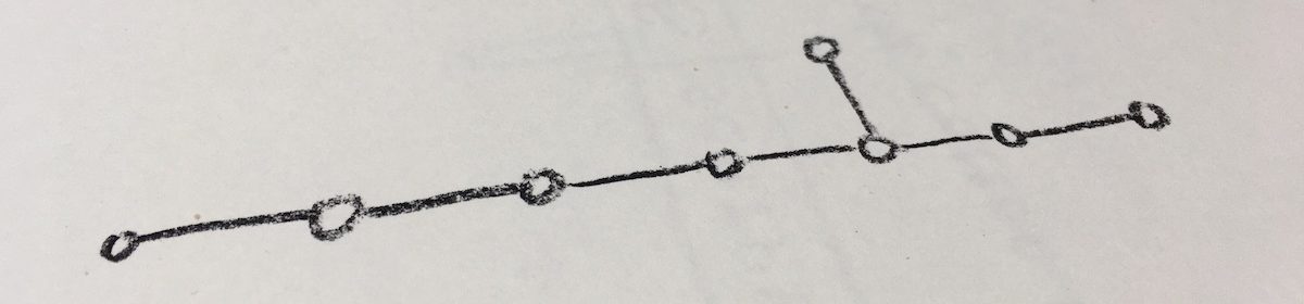

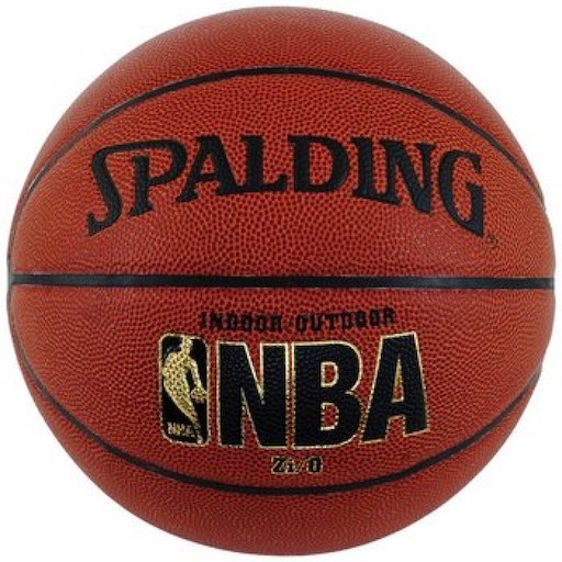

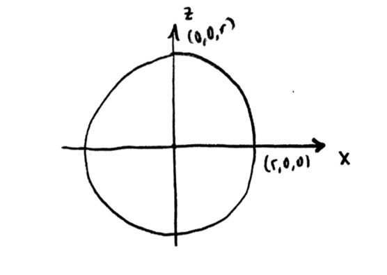
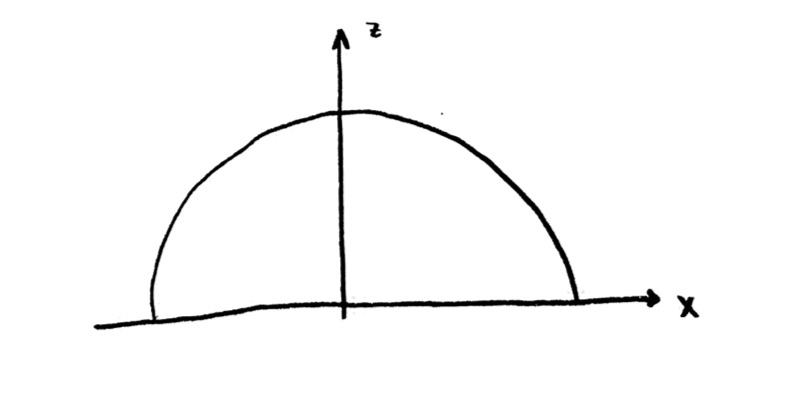
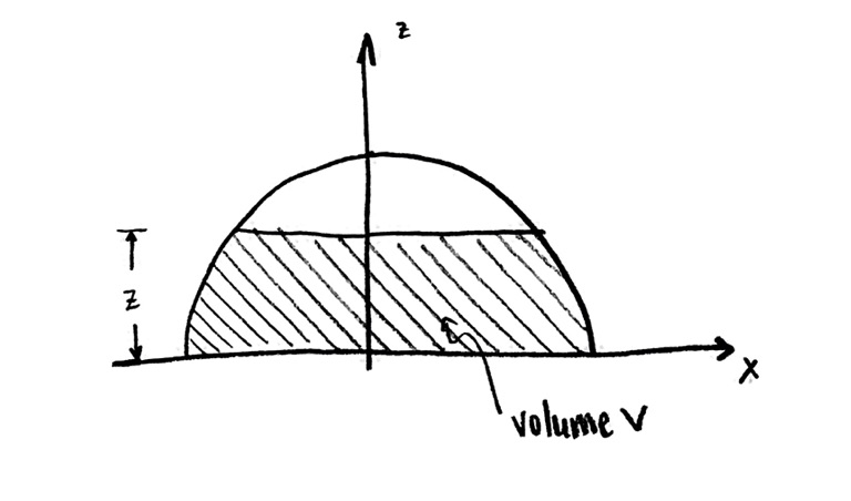
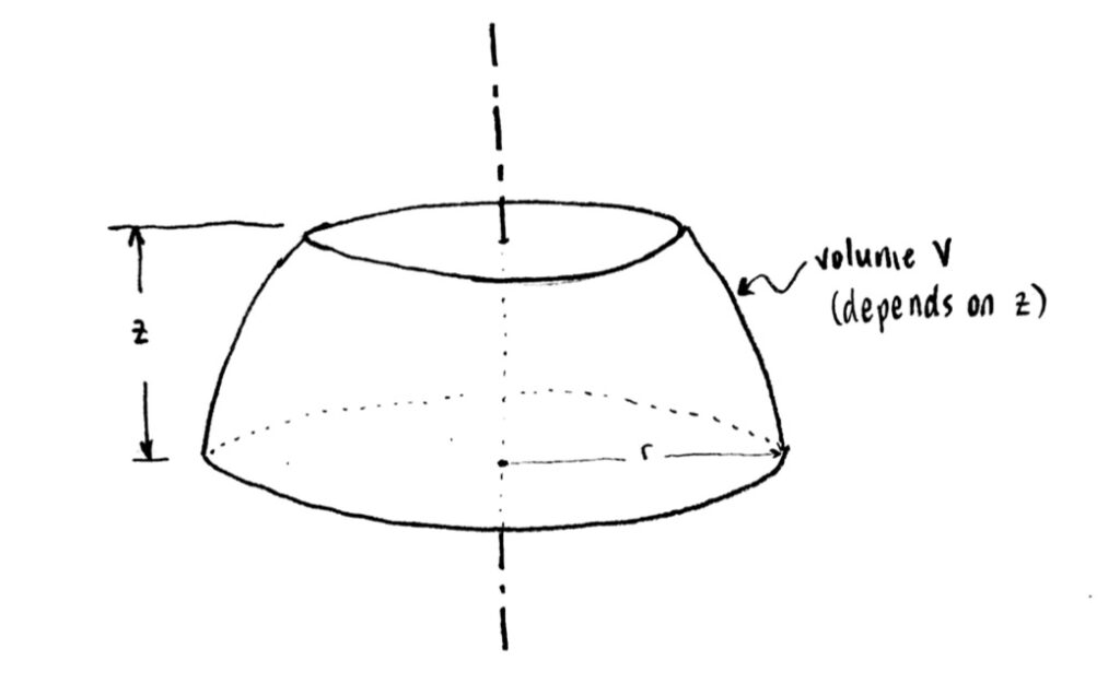
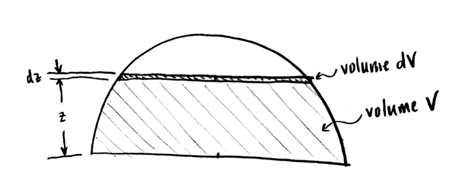
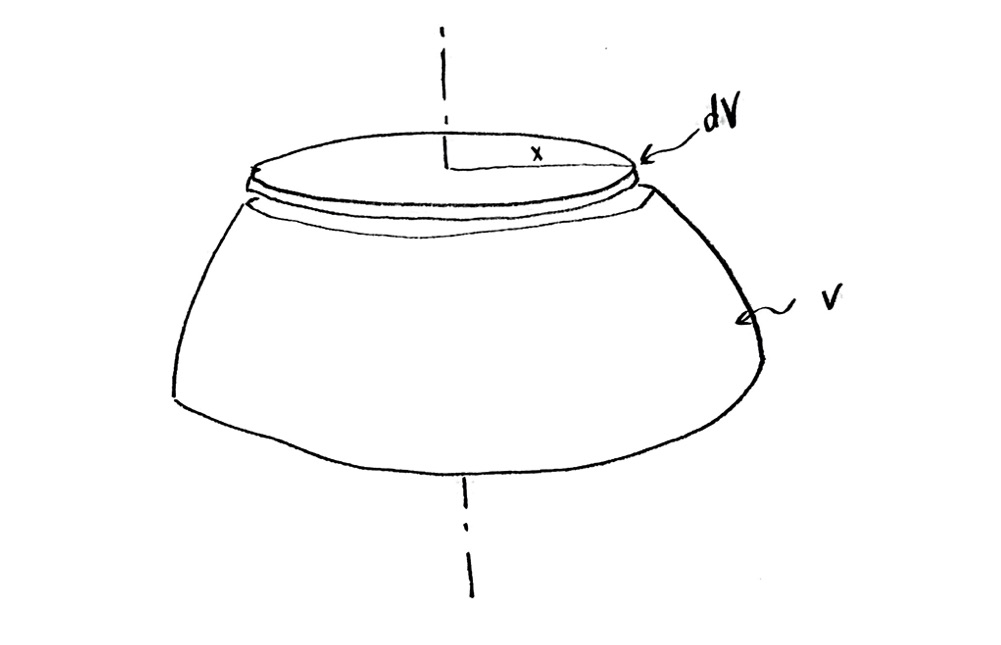
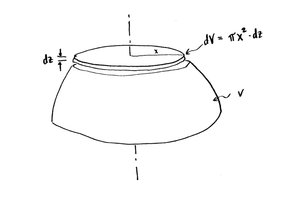
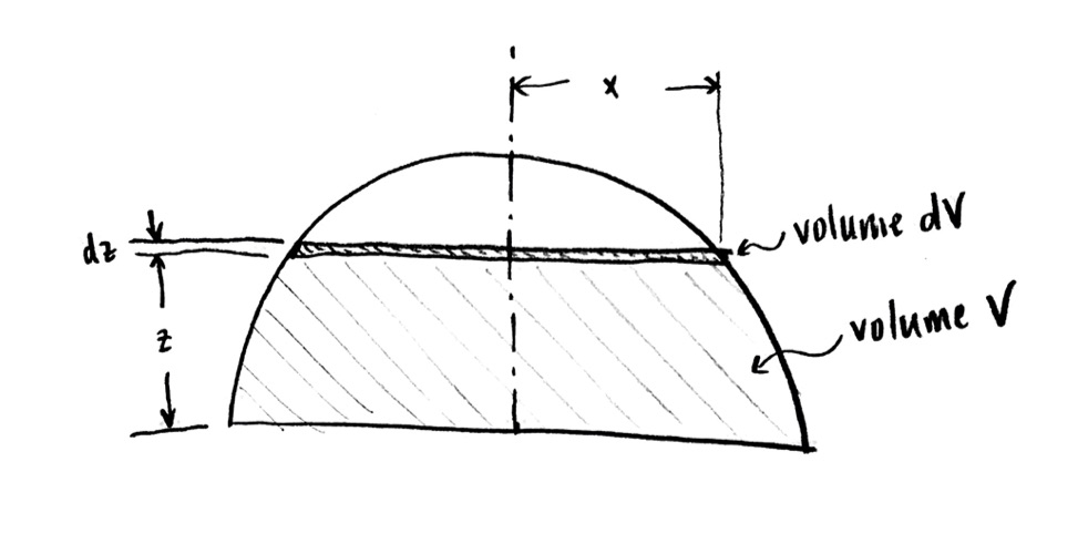
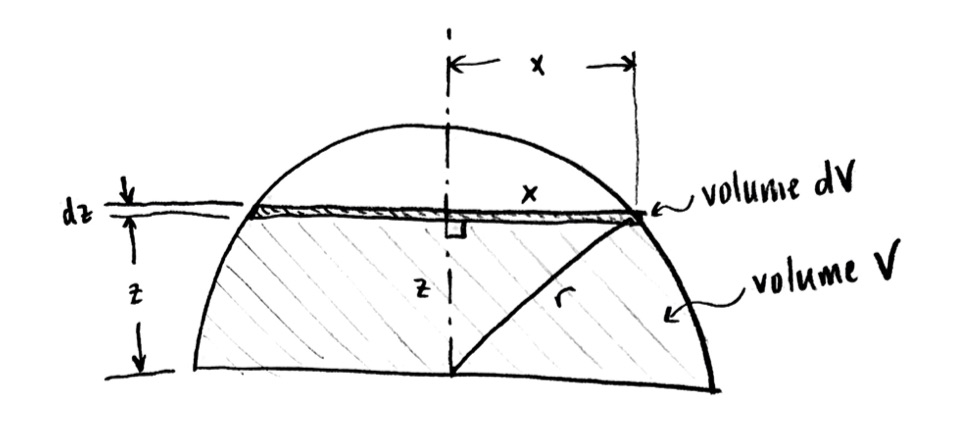

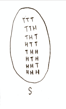
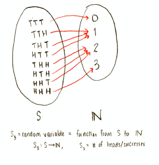
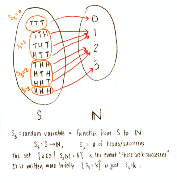
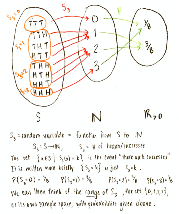
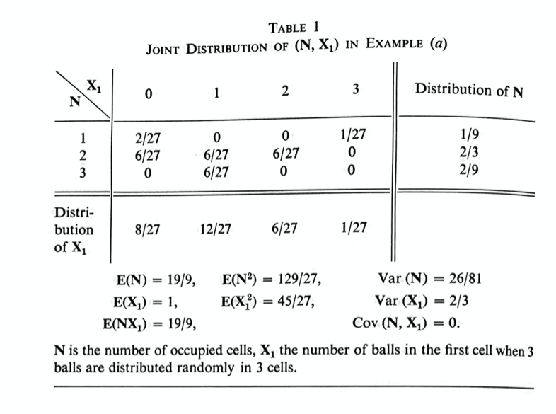
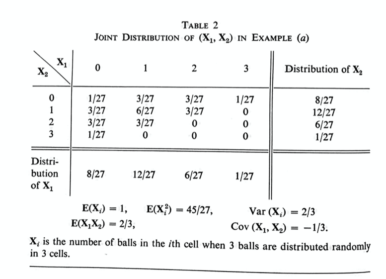

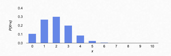
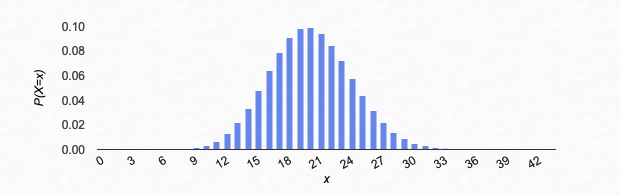
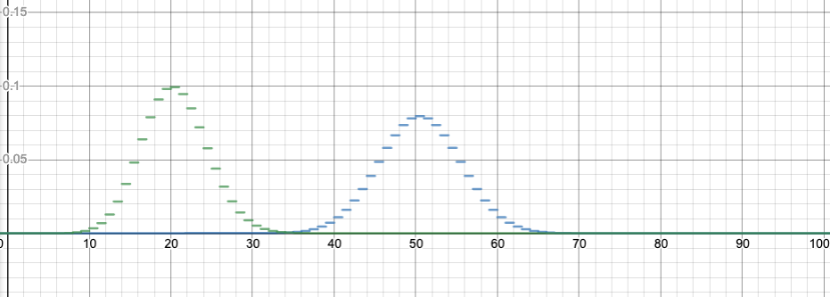
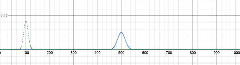
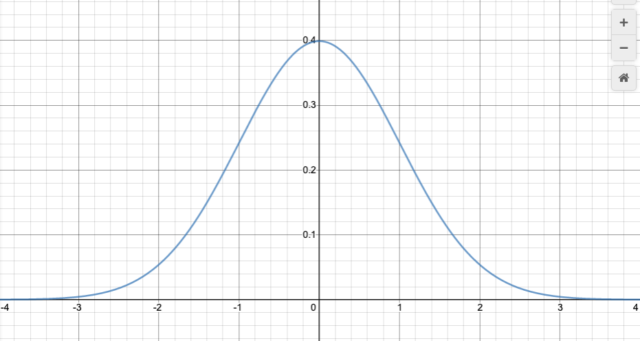
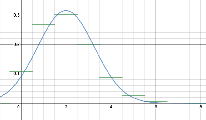


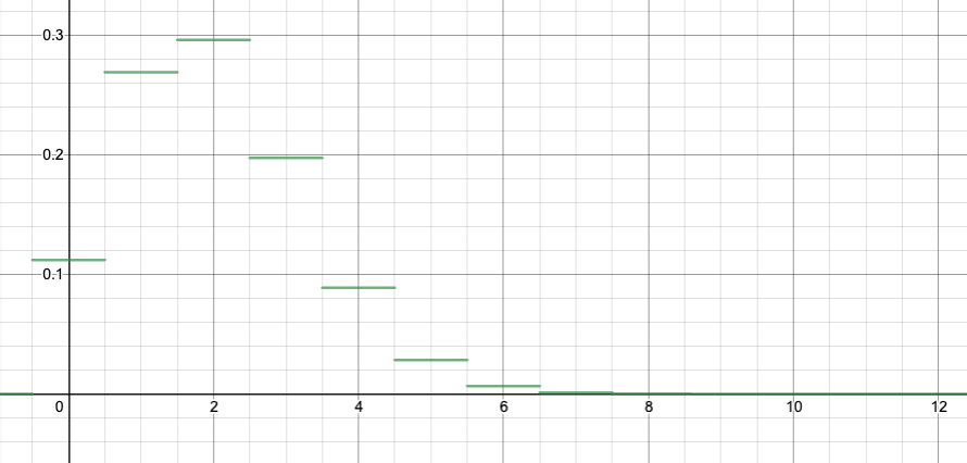
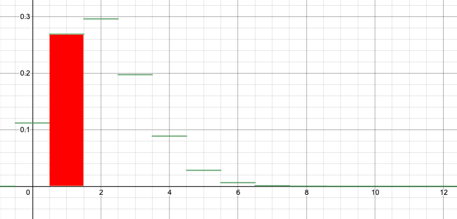
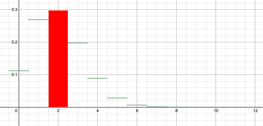

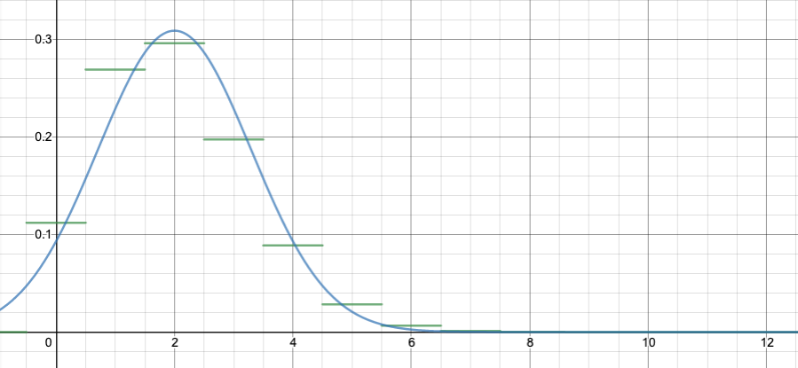
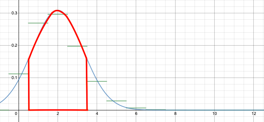
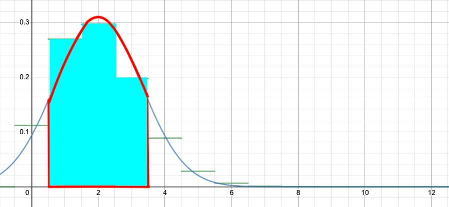

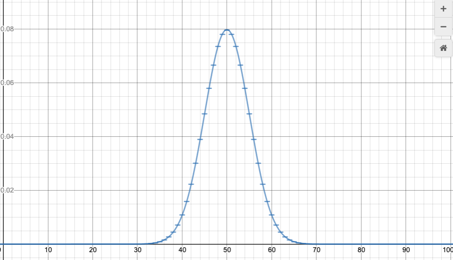
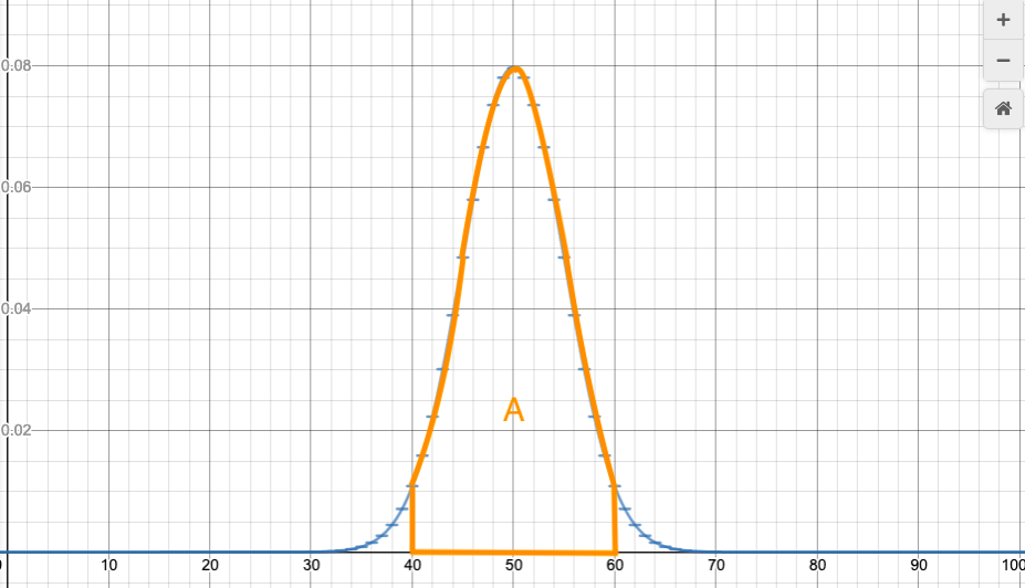
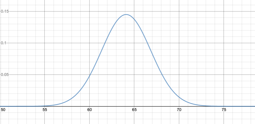
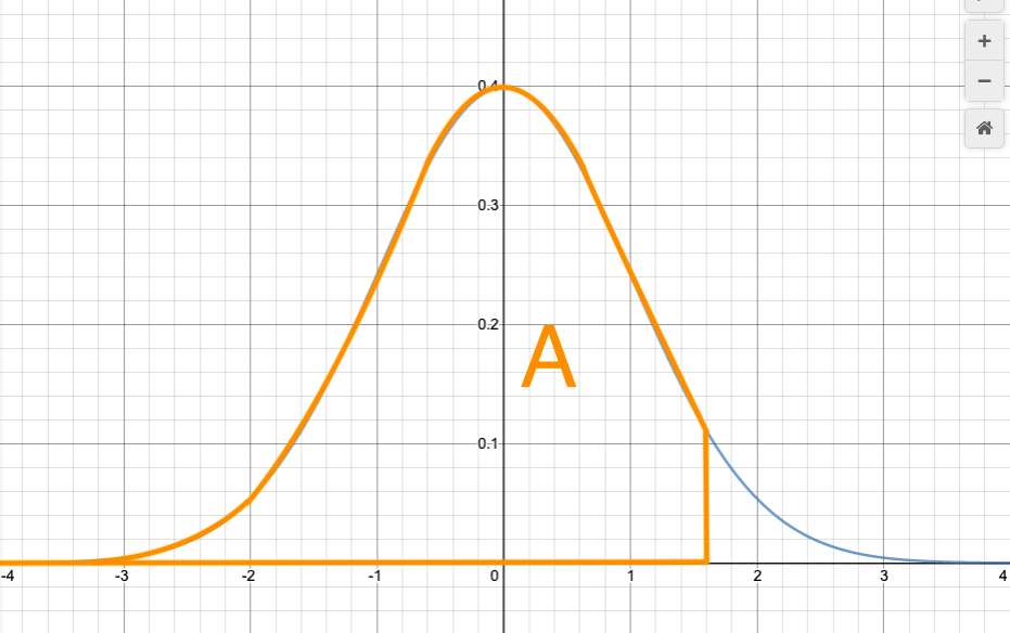
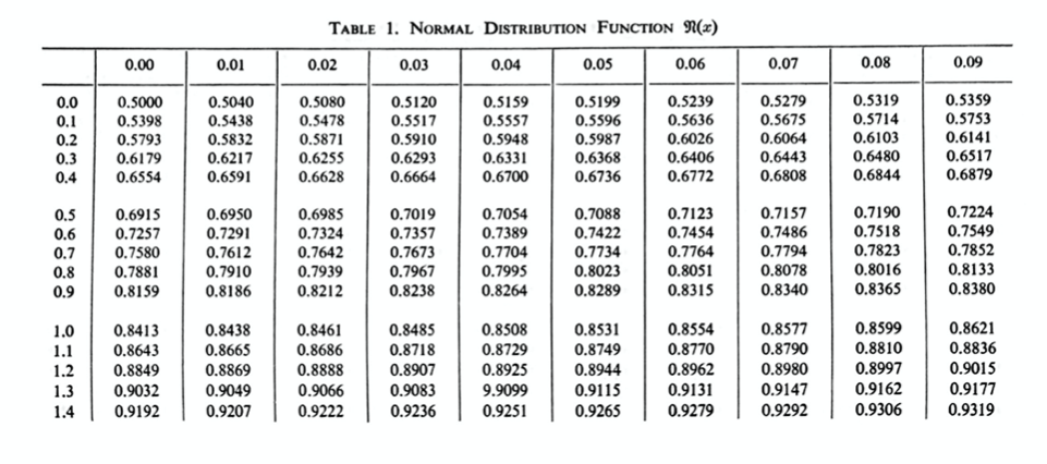
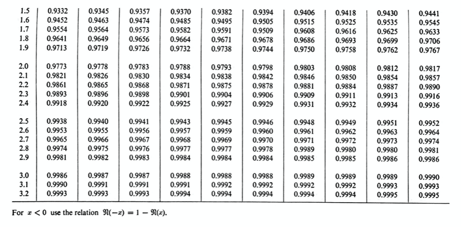
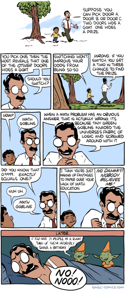
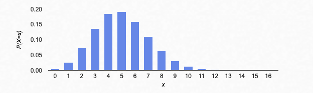

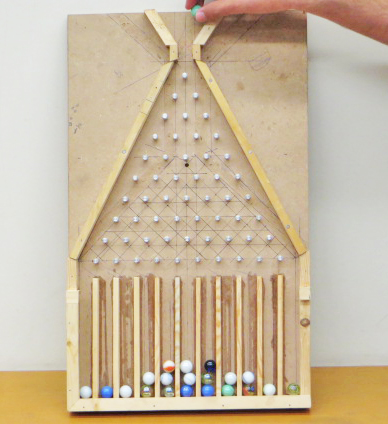
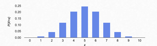
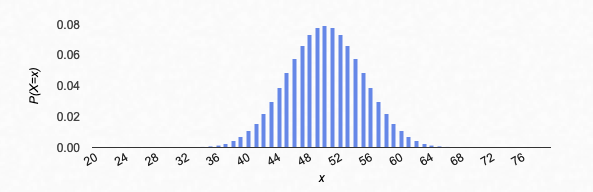

![xkcd comic. [lightning flashes]
"Whoa! We should get inside!"
"It's okay! Lightning only kills about 45 Americans a year, so the chances of dying are only one in 7,000,000. Let's go on!"
Caption: "The annual death rate among people who know that statistic is one in six."](https://mcintyre.bennington.edu/wp-content/uploads/2020/08/xkcd-conditional_risk.png)
![xkcd comic.
Did the Sun just explode?
(It's night, so we're not sure.)
"This neutrino detector measures whether the sun has gone nova."
"Then, it rolls two dice. If they both come up six, it lies to us. Otherwise, it tells the truth."
"Let's try. Detector! has the Sun gone nova?"
"[roll] YES"
Frequentist statistician:
"The probability of this result happening by chance is 1/36=.027. Since p<0.05, I conclude that the sun has exploded."
Bayesian statistician:
"Bet you $50 it hasn't."](https://mcintyre.bennington.edu/wp-content/uploads/2020/08/xkcd-frequentists_vs_bayesians.png)