OK, let’s start with the written lectures again! I’m going to try to keep this up for the rest of the term, if I can.
I would like to start these lectures beginning with our “reset” the other day. I’m planning to begin with topology with the cylinder and the flat torus (which we’ve talked about some already in class), and to go forward from there. But before I get to that, I’d like to zoom out a bit and look at where we are going.
Talking to you all in feedback meetings this week, it became clear to me that this would be a good moment to talk about the bigger picture again, before getting back into details. In particular, Sky articulated her questions in a very precise way, that made me see what I wasn’t communicating. I think several of you were having the same thoughts, but I wasn’t quite hearing it.
So, in this lecture, I want to talk about three things: 1) what I’m expecting you to do in this class; 2) what this class is about; and 3) what is math anyway? I’m going to take them in reverse order.
What is math?
I think that one puzzlement, lurking in the back of some of your minds, is this: when do we get to the real math? Where are the numbers, the equations, the fancy l0oking symbols? It was maybe a little clearer with the trigonometry and the Heavenly Mathematics text, where things looked a little more familiar. But in spherical geometry, and now topology, what is the point of all the pictures? Where is it going? When do the numbers and formulas arrive?
There is another question I think some of you have, which is actually closely connected to the first one: why all the writing? Why am I pushing you to write in a math class?
While it is true that a certain amount of math involves numbers and equations, there is a great deal of it that does not; or, at least, that is not the main point of it. The main point, in most advanced mathematics, is using logical argument, to understand the nature of the things you are studying. In this class, we are trying to understand the properties of shapes in various spaces (I’m using Sky’s wording here).
I almost said “the main point in most modern math” above. But in fact, in most of the earliest complete mathematical text we have, Euclid’s Elements, there are no numbers at all. Even angles are not measured (though the Greeks did use degrees as we do): Euclid says, for example, that the interior angles of a triangle add up to “two right angles”. (Euclid does have a couple of chapters on numbers, but he mostly banishes them from his treatment of geometry.)
One central idea of the Elements is to start with some very basic assumptions about the nature of space—axioms or postulates—and to logically explain the observed nature of shapes in space, starting from those very basic assumptions.
For example, the Egyptians were well familiar with Pythagoras’ theorem ( for the sides of a right triangle), more than a thousand years before Pythagoras; but we don’t have any record from them of why it is true. This is an empirical property of physical lines in space; Euclid shows that, based on a few fundamental assumptions, that it is a logical necessity. (Incidentally, Euclid manages to say Pythagoras’ theorem without numbers or measurement too!)
What does math look like?
Since Euclid is trying to make logical arguments about the nature of shapes in space, the Elements consists of diagrams, and prose arguments about those diagrams. Here is Euclid’s proof that the internal angles of a triangle add up to two right angles. (I am not expecting you to read this! But you can if you like!)
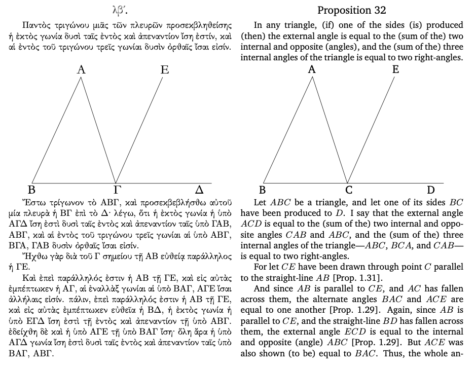

Note that it is a prose argument!
Note also that Euclid refers to previous things he has established; each assumption he makes, he justifies based on simpler assumptions, back all the way down to his fundamental postulates. The whole of Euclid reads as an interconnected story, where he assembles small pieces out of the most simple elements, then assembles larger and larger pieces out of the smaller ones.
Let me compare some modern math for you. Here is a page from my favorite graduate level general topology textbook, General Topology by John L. Kelley:
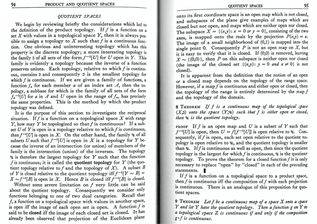
I’m definitely not expecting you to read that one! (The page I showed is talking about “quotient spaces”, which is something that we will get to soon, relevant to the torus and to “Torus Games”.) Note that there are some symbols, but most of it is logical argument in prose. Moreover, the symbols are part of the prose; every equation is part of a sentence.
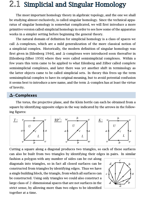
Here’s another example. This is from another classic graduate-level topology textbook. (Again, not expecting you to read it! Among other things, on this page the author is defining the torus and the Klein bottle as we have done in this class.)

I don’t want to oversell my point here: there are many areas of math which are about numbers and equations, and in which symbolism plays an important role. But even there, the equations are in the service of trying to understand the nature of things. And the tool for understanding the nature of things is logical argument.
I should also be clear that math is not about logical argument in quite the same way that, say, a political science paper is about logical argument. Although it is prose argument, math aims to talk about things which we can define very precisely, and make very certain arguments about. (More on that later in the class!)
What do mathematicians care about?
The Greeks probably considered Euclid’s postulates as self-evident truths about the world. In the nineteenth century, mathematicians developed new systems of geometry, with different assumptions than Euclid’s, which were nevertheless internally consistent, and beautiful. These systems were initially created in response to some unsolved questions from Euclid, but they soon took on a life of their own.
The attitude about postulates or axioms changed. (Note: I am taking “axiom” and “postulate” as synonyms; “axiom” is the more common modern word, but tradition has solidified “postulate” when we talk about Euclid.) People started to see the axioms as a set of assumptions which defined a mathematical system: a universe of thought. Different assumptions, different mathematical system. Different universe.
The relation of mathematics to the physical world was refined: a particular mathematical system could be taken as a model of the real world. Depending on what aspect of the real world you were trying to describe, one mathematical model or another might be more useful.
Euclidean geometry is an excellent mathematical model for the nature of lines, circles, and shapes made out of them, in the real world, provided we idealize the real world, (for example there are no true infinitely small points), and provided we keep the size of things small. When we get up to the size of solar systems and galaxies, for some purposes, a different geometry provides a better model.
(I said before that Euclid proves Pythagoras’ theorem, and that this establishes it as a logical necessity of how lengths in the real world work. That’s how the Greeks would have viewed it, but it’s not quite true. The way we would say it today is: if lengths in the real world obey Euclid’s postulates, then they must obey Pythagoras’ rule. Or more quantitatively, lengths in the real world obey Pythagoras’ rule to the extent that they obey Euclid’s postulates.)
That doesn’t invalidate Euclid though; Euclid is a perfectly good description of the nature of shapes in a particular mathematical universe, which Euclid defines through his postulates. As mathematicians, we can happily study the Euclidean universe. We still learn neat new things about it from time to time, and we use it when studying all kinds of other mathematical systems.
So why study different mathematical universes? Well, they may be useful for all kinds of things. But the more common reason is an aesthetic one. People are interested in unsolved problems in a given universe, like Euclid’s geometry. Mathematicians are often driven by unsolved puzzles. In the process, they are sometimes motivated to create new universes, which bend or modify the rules of the old ones. Then the question arises: how do things behave in this new universe? And, is this the only possible universe of this type? What are all the possible universes of a given type?
I would note also that mathematicians are often driven by aesthetic considerations. They want to understand why things behave as they do, they want to understand new universes, but they also want the explanations to be elegant, and the universes to be natural, interesting, and cool (all subjective judgments!).
A little more history
For a long time, one of the unsolved problems of math had to do with Euclid’s elements. Euclid has five postulates; four very simple looking ones, and one complicated looking one:
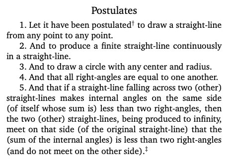
This isn’t necessarily a real problem, but it really bothered some people. For a long time, people wanted to prove the fifth postulate (named the “Parallel Postulate”), assuming the other four postulates. (Or, perhaps, to assume some simpler looking postulate in addition to 1-4, and prove 5 from the new set of assumptions.)
It’s a long story, but here’s a short version: in the early nineteenth century, several people were trying to prove the fifth postulate by contradiction. That is: let’s suppose the fifth postulate was false. Then, let me derive conclusions from that. If I can derive a conclusion that is obviously wrong, then my starting assumption must be wrong. Ergo, since my assumption that the fifth postulate is false is wrong, then the fifth postulate must be true! This is also called a reductio ad absurdum argument.
What these people very gradually realized is that, instead of reaching a contradiction, they were deriving results that were crazy-looking, but all perfectly self-consistent. They were describing a new mathematical universe, with different assumptions, in which the fifth postulate was false!
(In the process, they ultimately showed that the quest to prove the fifth postulate was in fact doomed: you can’t prove postulate 5 from postulates 1-4, because there exists a self-consistent universe in which postulates 1-4 hold, and postulate 5 does not!)
This new geometry was called hyperbolic geometry, and we are going to be studying it soon.
(In retrospect, spherical geometry is also such a new universe! And people had been studying spherical geometry for a lot longer, since the Greeks. People didn’t see it that way at first, in part because, depending on how you interpret them, postulates 1-4 aren’t quite true for spherical geometry. In the process of figuring this stuff out, people had to reassess what they meant by a “geometry”, and they had to restate Euclid’s postulates and proofs in more precise way. We’ll be getting to this soon!)
What is this class about?
Over time, the line of inquiry I described above merged with some other lines of inquiry that were coming up in other parts of math at the same time. Together, they suggested that new interesting territory was opening up, and this opened up three questions:
- What sort of local geometries are possible? For example, in a neighborhood, 2D space could look like a section of the Euclidean plane, or it could look like a section of the surface of a sphere, or it could look like the neighborhood of a vertex of the cube, or, or,…. Hypothetical flat beings that lived in this universe could measure the curviness of their universe by, e.g., measuring angle sums of triangles, or measuring circumferences of circles. What are all the possibilities here? How can a space be curved? And what are the properties of triangles, circles, etc in such a space, analogous to Euclid?
- What sort of global topologies are possible? On a cylinder, as we have seen, if you are in a small enough region, there is no way you could tell that your universe was not Euclidean. The local geometry is identical to that of Euclid. And yet, as a whole, the space is glued together differently. What are all the possible ways that a space could be glued together? How do shapes behave in such a space?
- How are questions 1 and 2 related? They way that the sphere is curved locally seems to be tied to the fact that it curls up into a ball shape globally. Can we say more here? For example, can we say anything about the average local geometry of other ball-shaped spaces (like a polyhedron, or an egg, or a football)? Will they necessarily be different from the geometry of donut-shaped spaces, like the flat torus?
That’s what this course is about!
In particular, all of our discussion of spherical geometry at the beginning came under topic 1 above. I wanted to show you a geometry whose local properties were different from Euclid’s, and I wanted to derive some properties of it. Then, I started us looking at trigonometry, because that will allow us to understand the behavior of shapes on the sphere a lot better. There are still some very cool things about spherical geometry we still have to get to! The study of polyhedra also comes under topic 1: we were trying to figure out the local geometry of such spaces, e.g. how triangles and circles behave.
Right now, we are putting the sphere on hold, and pausing topic 1, in order to start investigating topic 2. The torus is one example of how space can be glued up to itself, in a global topological sense.
There isn’t a super clear dividing line between 1 and 2. We are studying the torus; but Weeks and I are insisting on studying the flat torus, which is prescribing a certain sort of local geometry on that torus. (If we picture the torus as the surface of a donut shape sitting in 3D, that is topologically correct, and helpful, but it is geometrically misleading, because the flat torus is not locally curved, whereas the donut shape is locally curved. More on that soon.)
My goal, since the reset, is to work seriously on topic 2 for a bit, and then link it back into topics 3 and 1.
What I want you to be doing in this class
My goal for this class is partly to take you on a tour of these ideas. But it is also partly for you to try to work through the ideas as mathematicians would. I want the class to be as authentic an experience as possible of doing mathematical research, as people have done it historically, and as people are continuing to do it today.
In mathematics, the word “research” means something different than it does in other subjects. It doesn’t mean looking up articles, although that can be part of it. It means this sort of exploration: creating new universes, figuring out how they behave, figuring out what universes are possible. Making conjectures about what is true, and then trying to prove the conjectures, or to find counterexamples.
That means that I am asking you to explore the ideas: how does this new universe behave? What are the properties of shapes in it? The new universe is going to allow things that weren’t an issue in Euclidean space; what should we allow in our definitions? Can we extend what we know to the weirder possibilities in some consistent way, or no?
I think that, 1) this process of doing mathematical discovery is fun and interesting, and should not be limited to only those few people who go through graduate school in math first; and 2) that, even if your goal is only to learn more basic mathematics, this is the best way to do it. Figuring things out yourself, and figuring out why they are true, gives you more fluency and understanding than just taking formulas from a book and applying them. (And getting in this habit makes you better at reading math: reading a math text becomes more of a collaboration between you and the book, rather than just accepting things passively.)
So that’s the reason behind the open endedness of many of the questions I’m asking. I’m not being ambiguous just to be annoying. I’m trying to ask: what questions are natural to ask here? What is interesting? What is a fruitful way of summarizing and organizing what we have figured out so far? I’m hoping that you will explore, and in particular that you will formulate your own questions, and try to answer them.
Writing solutions, and notebooks
This is also the reason behind my encouraging you to write more words, and to work in a diary format. You are writing a field notebook, for exploring new universes. It’s true that your initial rough work, as you are starting to explore new territory, will look like a crazy collection of drawings and scribbles and numbers. But it’s important to try to organize your thoughts, and to be clear about where you are trying to get to, what you’ve figured out so far, and what is holding you back.
Let me show you an example. Here are a few excerpts of pages of personal notebooks from a mathematician, Dan Quillen. The math words aren’t going to make any sense to you, but I’d like you to note the style. First, he has made an index page at the front of each book (which is filled in as he works in the book):
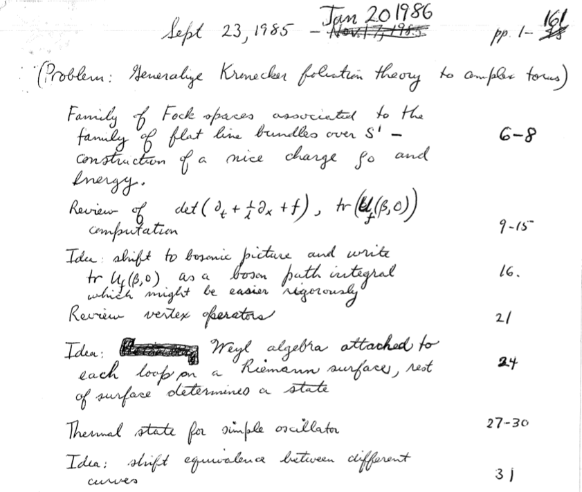
Some things are labelled “ideas”, that he wants to follow up. Other things are reviews, reminding himself of what he knows (or is learning).
When he starts thinking about something, he sets up what he wants to do:
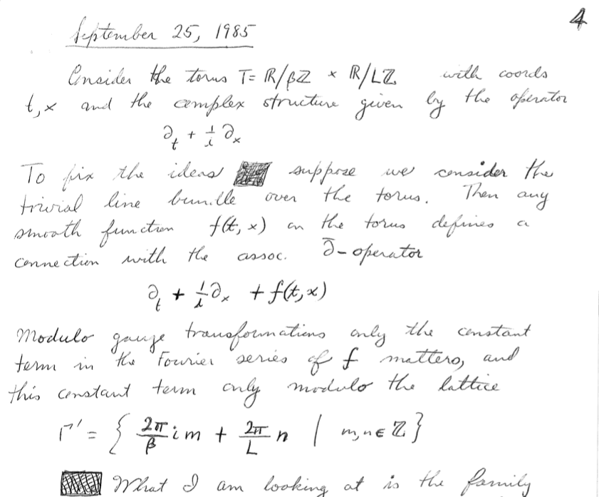
Note that there are symbols, but the symbols are always parts of sentences.
He talks about where he is getting stuck, and tries to explain to himself why:
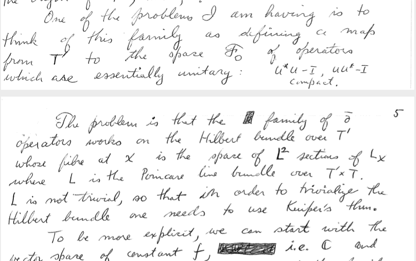
He’s making plans, and making guesses about what he hopes might be true, sometimes in a vague sense:
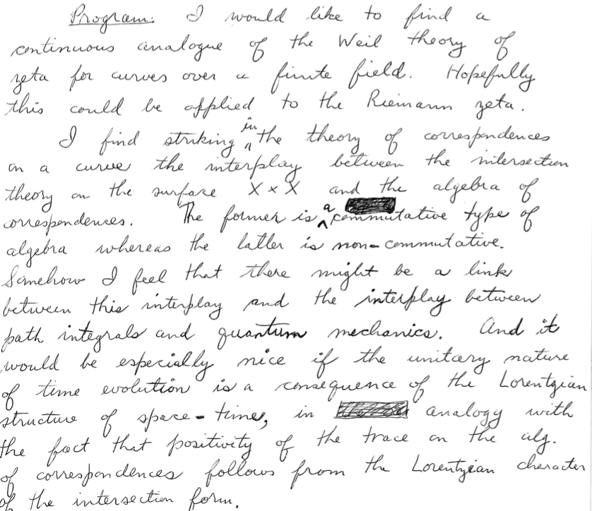
“Somehow I feel that there might be a link…” “And it would be especially nice if…”
You can find scans of all of Quillen’s notebooks (!) here.
Full disclosure: not all of us keep notebooks this carefully! But I know that when I do, I make better progress. And that when I don’t, I often come to regret it, when I’m trying to decode my weird scribbles later on.
Collaboration
Another important element of this authentic experience of mathematical research and exploration is collaboration. While there are some mathematicians who work alone, and while some work is always done on one’s own, it is more and more the case that most mathematical work is done collaboratively with others.
This has the advantage that your collaborator’s strengths may be your weaknesses, and vice-versa. It is helpful to try to explain your thoughts to another person. It is helpful to listen to another person’s thinking and to try to make sense of it. When you are feeling stuck and lost, it’s easier to keep going when someone else is stuck and lost with you. And it’s often more fun!
Especially in this moment, when we are all separated and communicating virtually, I think this process of talking to each other and working together is important. I would therefore strongly encourage you to try to find people you like to work with. Talk to me and to Sophia, but also talk to each other. Talk in Slack in the open channels, and then direct message someone if you want to have a one-on-one conversation. Think of someone you liked working with in class, and DM them on Slack. Either text through Slack, or make a call (which you can also do on Slack, just click on the person’s name). Put your profile picture up on Slack, so that someone who remembers working with you from class, but who doesn’t recall your name, can find you.
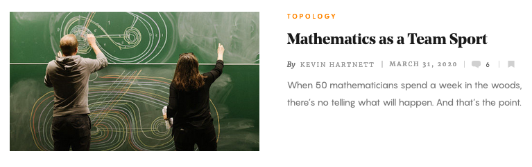
To give you an idea of what collaboration among math professionals is like, I’d like you to read the article I have linked below. Coincidentally, it also happens to be about the subject of our course! The type of topology that the people described in the article are doing is an outgrowth of what is in Shape of Space. (There was a mathematician working in the 1970s, Bill Thurston, who brought in a lot of new ideas. Jeffrey Weeks, the author of Shape of Space, was his student; many of the people described in the article are either Thurston’s students, or students of his students, or students of students of students. I’ll say more about this later!)
What next?
Well, that was all more than I had started out intending to say! In the next lectures, I’ll get back to the specifics of the torus and the cylinder, make some hints for the problems, talk about intrinsic vs. extrinsic geometry, and introduce the Möbius strip and Klein bottle.
 : the number 1,000 consists of 3 factors of 10. That is:
 means
means  , and
, and  means
means  , and
, and .
. means x = log (y) (2)
 (3)
(3) (4)
(4) . For any number x, the number log(x) is “how many zeroes are in x”; then doing
  is making a number with exactly that many zeroes, which is just x!
 and
and  (D)
(D) (E)
(E) .
.
 (by (M))
 (by (4))
 (subtracting log(3) from both sides)
 (multiplying both sides by 3.55)
 (I’m estimating in my head, you can use a calculator for more accuracy)
 ,
, (taking logs of both sides)
 (by (M))
 (by (4)),
 .)
.) for the unknown x.
 for the unknown t.
 ,
,  , and
, and  are some known quantities. Suppose we know the equation
  holds. Solve this equation for t. (Your answer should be a formula for t, which will depend on
  of both sides.
  . I want to solve this for the unknown x. I start by using regular algebra to solve for the log x:


 ,
, .
. .
. ,
,  , and
, and  are known numbers, and suppose we know that the equation
  is true. Solve this equation for the unknown x. (Your answer should be a formula for x, which involves the
  . Now, instead of graphing y, I am going to graph the values of
  . Let’s give this new variable a name; say
  . Taking logs of both sides of
 (by (E))
 , where z stands for log y, and m stands for log 2.
 .
. .
. , where a, b, and c are some constants, x is the input, and y is the output. Convert this to an equation for log y as a function of x. Simplify as much as possible. Then, describe what the graph will look like. Be as specific as you can: for example, if it is a straight line, say what its slope and y-intercept will be. (Your answers will be formulas depending on the constants a, b, and c.)
 individuals, at the initial time
  .
. is true:
 .
. .
. .
.

 ,
, .
.

 .
. ;
;

 .
. to prove the division rule for logarithms shown above.
 ,
, ? Well,
  (13 times),
 .
. ,
, .
. , I could observe
 ,
, , so
, so  . (The exact answer is 8,192. If we had log tables and used pencil and paper, we could get a lot closer.)
 .
.
 , in other words,
  .
. . So
. So 
 .
. . So
. So .
.


 . But what is special about 10?
 ; the log base b is written
  . One exception: usually for
  , people instead write
  , which stands for the “natural” logarithm. The default assumption is 10, so if we write just
  it means
  ; sometimes people write


 , which is approximately 1.414, or more roughly, about 1.4. So a half of a two is about 1.4. As we did before, we could use that to estimate some other logs. For example, since 90 is approximately 64 x 1.4,
  .
. . (Right? Review it now if you need to. I’ll wait. … OK, you’re back? Great.) That is to say, a two is worth about 0.3 of a zero. More mathematically stated,
  .
.  ,
, ,
, . We need an extra 0.1 of a zero, that is, an extra
  . But that is one third of a two, because
 .
. .
.
 ,
, .
.
 : you take the log base 10 of the number, multiply it by 3, and then add one third of that number. For example, to find
  , I would first find
  , which is about 2.55 (remember why?? Do it now!). Then I would calculate:

 ,
, . Given the relationship between the two types of logs, how would the graphs be related?
 is about 0.3, this means that a two is worth about 0.3 of a ten:
 .
. .
.

 ,
,

 .
. .
. ;
; .
. .
. ;
; ,
,


 .
.


 .
. . In other words, that defines what we mean by
  . Why the 2? Well, historically, people tended to work with the diameter rather than the radius, so they wrote this formula
  , or equivalently
  .)
.) radians (for math reasons we will see as we go on).
 and
and  respectively.
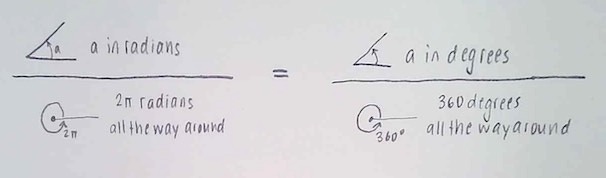
 .
. is equal to
  (try it!).)
 ,
, .
. , I automatically read it as
  (which is standard in advanced math).
 ,
, .
. . More simply, I just read
  automatically as meaning
  , basically by definition.
 .
. .
. in terms of
  .
. radians to degrees. Don’t use the formula you worked out; instead, go back to the proportions and work it out from there. (Hint: You’ll get a fraction over a fraction at first. But rewriting the big fraction in the way I recommended will eliminate this potential problem.)
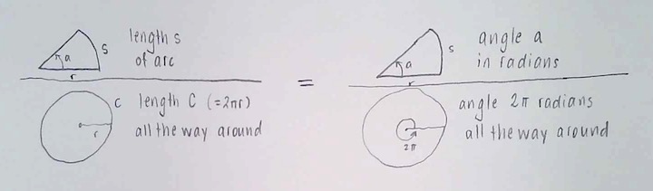
 ,
, .
. .
. radians.
 means multiply 10 by itself, x times:


 . (And if you recall our discussion about that, the number that has exactly half a zero is the square root of 10:
  exactly.)
 ; checking on a calculator, we find that
  , to four decimal places. So the number 6.3536 contributes 0.8030 zeroes; we could write
 ,
, ;
; ). (Right!? Check my math!)
  ) number of working people, each making 4.5 zeroes (
 ) dollars each per year. For total dollars made per year, you multiply; but multiplying adds zeroes. So the total income is 8.3 + 4.5 = 12.8 zeroes worth of dollars per year,
  dollars per year.
 , that is, I should add 0.5 zeroes.
 dollars. Now, 12 zeroes is a trillion, and 1.3 zeroes is about 20 (why?), so I get an estimate of
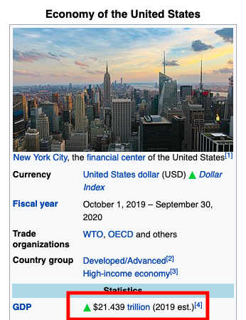
 or
or  , so our brains never have to manage numbers bigger than 80 (and usually smaller ones). For another thing, in problems like this, we are almost always multiplying, which is difficult both for doing mentally and for having an intuition. But number of zeroes (the logarithms of the numbers) add rather than multiply. Adding is easier.
 .)
.)

 , and multiplying numbers adds the number of zeroes. The logarithm counts the zeroes, so
  . (Actually a little less than
  , because if 3 was exactly half a zero, then 3 x 3 would be exactly 10.)
 ,
, ,
, ,
, by the fundamental rule:
 ,
, .
. ,
, ,
, ,
, . It is not exactly
  ,
, ,
, .
. .
.
 , and
, and  , so I’m going to guess that
  . This finally leads to the estimate
 .
.
 , as above, but remember
  , and figure out the other values from these.
  and
and  …)
…)