Hi everyone!
This follows the lecture on Differential Equations.
This lecture combines two things: I will give some more examples of setting up a differential equation model, and graphing the slope field.
I will also ask you some problems, which I would like you to submit, so I’m also going to call this lecture “Problem Set #8”. Please submit these problems, over slack as usual. You can submit them one at a time. Please indicate in the message the problem set and the problem name, e.g. “Problem Set 8: Numerically approximating the solution of a differential equation”.
I’m mixing the examples together with the problems so that I can explain the problems before getting you to do them, with extra examples as necessary.
Problem: Approximately numerically solving a differential equation
I’d like to start by getting you to do an example like in the previous lecture. In that lecture, I started with the difference equation
$\Delta P = (0.10) P \Delta t$,
describing population growth, at a 10% per time period rate.
At first, I took $\Delta t=1$: that meant that 10% was added to the population discretely, once every time period, and I tabulated it. That is a good population model if the animals have a definite breeding season, for example.
But then, I imagined that the reproduction was happening continuously. In this case, the population does NOT grow by 10% in one hour. Even though that is the continuous rate, after an hour, we will actually have more than 10% added!
That’s because, in that first hour, individuals were being added, and they contribute to the growth. For example, I started looking at half time periods, $\Delta t=0.5$. In the first half time period, the population would increase by 5%; those extra 5% would then reproduce in the next half hour.
But that’s not really good enough, if the growth is continuous: in that first half hour, individuals are added as well. So I split it into quarter time periods $\Delta t=0.25$, tenths of time periods $\Delta t=0.1$, . . . and tabulated those. (Look at the previous lecture to see what I’m talking about!)
Continuous growth would be the limiting values of that table, as I take the $\Delta t$ smaller and smaller. The limiting case would be a solution of the differential equation
$\mathrm{d}P = (0.10) P \,\mathrm{d}t$
or
$\dfrac{\mathrm{d}P}{\mathrm{d}t} = (0.10) P$
OK, I’d like you to try this yourself:
Problem: Numerically approximating the solution of a differential equation
Suppose we want to solve the differential equation
$\mathrm{d}P = P \,\mathrm{d}t$.
(I have replaced the rate $r=0.10$ in the example I did, with $r=1$ instead. So the organisms are reproducing at a continuous rate of 100% per time period.) Suppose that the initial population is $P=1000$ at time $t=0$. I want you to estimate the population after one time interval, that is, the population at time $t=1$.
As I did before, I’d like you to use the difference equation
$\Delta P = P \Delta t$
for smaller and smaller values of $\Delta t$.
a) Take $\Delta t=0.5$, and make a table which goes up to $t=1$, to estimate $P$ when $t=1$.
b) Take $\Delta t=0.25$, and make a table which goes up to $t=1$, to estimate $P$ when $t=1$.
c) Take $\Delta t=0.10$, and make a table which goes up to $t=1$, to estimate $P$ when $t=1$.
d) How far do you think I have to take this to get an accurate answer for $P$ at time $t=1$, when the growth is continuous?
e) Keep going, with smaller $\Delta t$, until you are confident that you have an answer for $P$ at time $t=1$ that is correct to the nearest whole number.
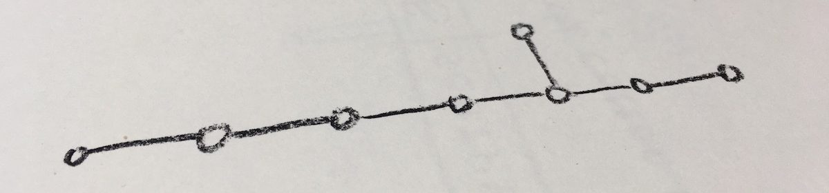
Problem: Nuclear Decay
OK, now I’ll ask you to cook up another model. This model will be very close to the exponential growth model that I described in detail in the previous lecture, so you might want to refer back to that lecture as you do this problem.
To set up the model, I have to explain a little about the physical system I’m trying to model.
We start with a sample (say a rock, or a piece of charcoal), that contains some number $N_0$ of unstable (radioactive) atoms. After some time, each atom will “decay”, meaning that it will release a particle of radioactivity, and the atom will transmute to a different element or isotope. Effectively, if all we care about are the radioactive atoms, then the atom which has “decayed” is no longer there (it has changed to something else), so the number $N$ of radioactive atoms is reduced by one.
How long a particular radioactive atom will take to decay is random and unpredictable! So it might seem hard to predict what is going on. However, the average time a radioactive atom takes to decay is very consistent and predictable. It’s a known number, which depends on the type of atom. And any reasonable size sample contains billions of atoms or more, so the randomness averages out pretty smoothly.
In a time period, a known number $rN$ of the radioactive atoms will decay, where $r$ is a constant proportion. Those atoms will be removed from the total.
But, like I discussed in the previous lecture, this is continuous process. So, for example, if I say that 10% of the atoms decay per hour, that is a continuous rate. It doesn’t mean that after 1 hour, the number of atoms will be reduced by 10%. For example, if we split it up by half-hours, then after one half-hour, 5% will have decayed—leaving fewer to decay in the next half-hour. And that’s not really good enough either: we should split it into quarter hours, or tenths of an hour, or minutes, or seconds. . . We should really look at the amount reduced in an infinitesimally small time $\mathrm{d}t$.
Problem: Nuclear decay model
a) Set up a differential equation that models nuclear decay. Let $N$ be the number atoms we have, at time $t$. Assume that the rate of decay is: 10% of radioactive atoms decay per time period. (But as discussed, that is a continuous rate, so there will actually not be exactly 10% in one time period.) Your answer should be very similar to the exponential growth differential equation from the last lecture, with only one key difference.
b) Draw the slope field, the same way I did for the exponential growth model in the previous lecture.
c) Although negative $N$ doesn’t make much sense for our model, extend the slope field to negative $N$ and negative $t$ anyway, just to see how it works mathematically.
d) Draw a typical solution curve to this slope field.
e) Does the shape of the solution curve make sense, in a practical sense?
f) What happens to the number $N$ of radioactive atoms after very long times, $t\to\infty$?
Some simple abstract differential equation examples
Now, I’d like to try a few simple abstract examples of differential equations. I’m not going to worry about what they’re modeling: I’m just going to set them up as straight math, to get some practice with the slope fields and solution curves.
Let me start with the simplest example I can think of. Let’s say $y$ is my function, and that it depends on the input variable $x$. I’m going to make a differential equation of the form
$\dfrac{\mathrm{d}y}{\mathrm{d}x} = \text{something}$,
which is the simplest form. (All my previous examples have been of this form so far.)
The simplest “something” I can think of is a constant. Let’s make up a constant, say
$\dfrac{\mathrm{d}y}{\mathrm{d}x} = 1$.
What slope field does this correspond to? Well, the differential equation is saying that the slope is 1. Always 1. Forever 1. It doesn’t even matter what $x$ and $y$ are. Differential equation don’t care. Slope is 1.
So every time I draw a little slope line, that slope is going to be 1:
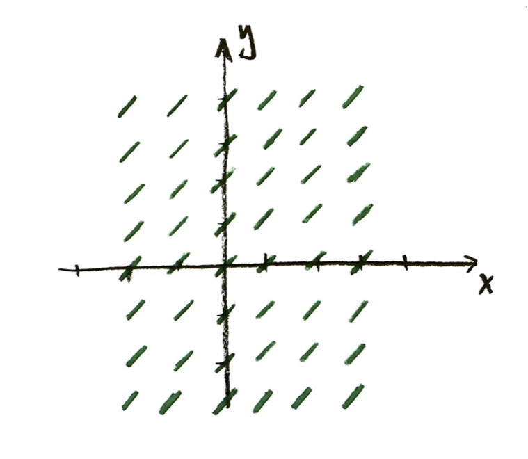
Nice!
What’s a solution curve for this slope field going to look like?
That’s right, it will just be a straight line:
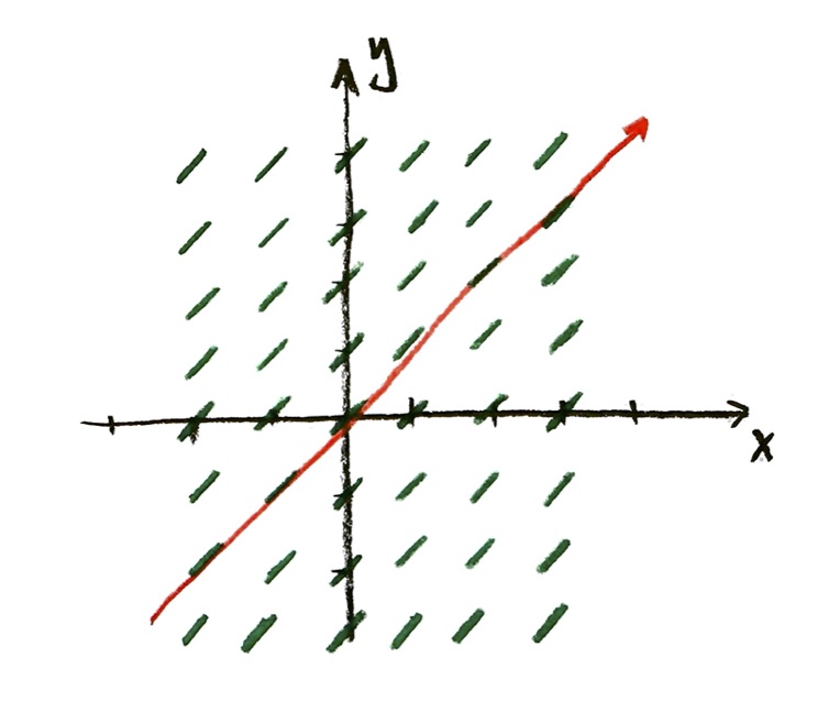
I drew the straight line starting at the point (0,0). But that was an arbitrary choice. I could have drawn the line starting at any point. Here are two more lines, one I drew starting at (0,2), and the other at (0,-1):
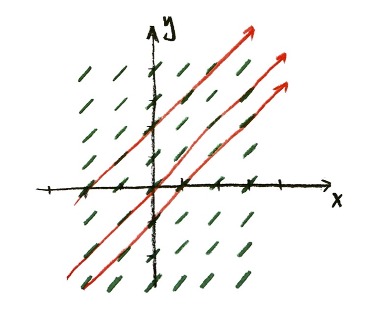
The choice of starting point is called an “initial condition”.
Now, this differential equation was simple enough that I can actually find an explicit formula for the answer! If
$\dfrac{\mathrm{d}y}{\mathrm{d}x} = 1$,
then a function with derivative of 1 would be
$y=x$,
or more generally,
$y=x+C$
where $C$ is any constant.
That agrees with my picture, right? The three solution curves that I drew were
$y=x$, $y=x+2$, and $y=x-1$,
corresponding to different values of the constant $C$.
What sorts of other slope fields do we get with this simplest example?
Problem: dy/dx = k, where k constant
Let’s say we have the differential equation
$\dfrac{\mathrm{d}y}{\mathrm{d}x} = k$,
where $k$ is some constant. (Our example above was $k=1$.)
a) What does the slope field look like, qualitatively? You should have three possible cases, depending on what sort of value the constant $k$ has . . .
b) Draw some solution curves in each of the three cases.
c) Write the general solution to the differential equation. (It will be the same equation for all three cases.)
Now, I’d like you to try the next to simplest example on your own:
Problem: dy/dx = x
Let’s say we have the differential equation
$\dfrac{\mathrm{d}y}{\mathrm{d}x} = x$.
a) Draw the slope field for this differential equation. (Pick some points, say (0,0), (0,1), (0,2) . . . then (1,0), (1,1), (1,2), . . . , then (2,0), (2,1), (2,2), . . . etc. At each point, use the differential equation to find the slope, and draw a little line with that slope, at that point.)
b) In (a), I suggested using points with positive values. If you didn’t do it already, extend your slope field to some negative values of both x and y.
c) Draw two different solution curves to this slope field.
d) Find the explicit equation of y as a function of x, that will solve the differential equation.
e) Check that your explicit formula agrees with the solution curves that you found graphically!
Let me show you another example, this one slightly more complicated. Let’s consider the differential equation
$\dfrac{\mathrm{d}y}{\mathrm{d}x} = y-2$.
Try drawing the slope field yourself first, don’t look at the answer, I’ll wait!
. . .
. . .
. . .
OK, what did you get? My slope field for this differential equation looks like this:

Is that what you got?
I got it by substituting points (0,0), (1,0), (2,0), (1,0), etc etc. in for x and y in the differential equation to find the slope. Then drawing a little line of that slope, at the corresponding point. For example, the little line at (0,0) has slope dy/dx = y-2 = 0-2 = -2.
But, I could do this more conceptually, since I just want a qualitative picture. First, I note that the slope dy/dx = y – 2 does not depend on x! So the slope lines will have the same slope if I change the x coordinate, that is, if I move horizontally. So the slope on horizontal lines is constant.
Next, I look at what happens vertically. An important value is y=2: if y=2, then the slope is zero. That’s significant, so I draw that first: a bunch of horizontal slope 0 lines, all along the horizontal line y=2.
Then, if $y>2$, I know that the slope dy/dx = y-2 is positive. So the slope lines above the line y=2 will all point up (going left to right). And, the more y is bigger than 2, the bigger that slope will be: the lines slope up more as I go up further above the line y=2. I draw all those in, remembering that the slopes are constant along horizontal lines.
Finally, if $y<2$, then the slope dy/dx = y-2 is a negative number. So the slope lines below the line y=2 will all point down (going left to right). Again, the further we are below y=2, the more negative those slopes will be.
OK, so what do solution curves look like? Let me start with one that begins at the point (0,3), above the line y=2:
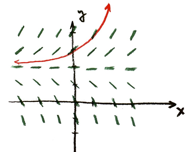
Note that I started at (0,3), and followed the slope field going in the positive x direction (to the right). But I also started at (0,3) and followed the slope field going backwards, in the negative x direction (to the left).
As I go backwards from (0,3) in the negative x direction, the slope field is pushing my solution curve down towards the line y=2. However, as my curve gets closer to y=2 for negative x, the slope line also gets shallower. I haven’t drawn them all, but as y gets close to 2, the slope dy/dx = y-2 gets smaller. So as I travel in the negative x-direction, the solution curve gets closer to y=2, but more and more slowly, so it never quite gets there. The technical word for this is that y=2 is an asymptote for the solution curve.
If I start below the line y=2, say at (0,1), then I get something kind of opposite:
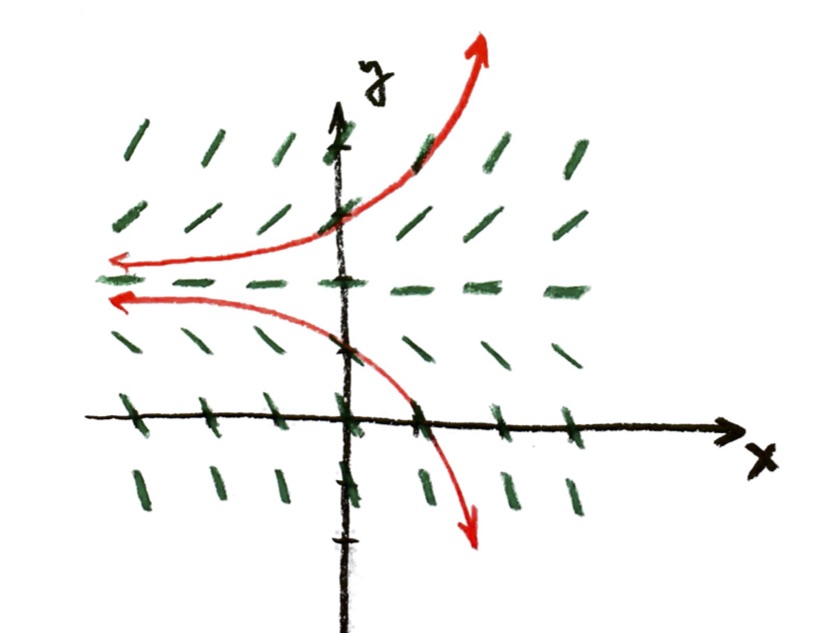
You should check the logic of that curve in a similar way.
There is one other possibility: if I start exactly on the line y=2, then I will (in theory) stay there forever, because the slope is 0, and the solution curve doesn’t move up or down:

The technical word for this is that y=2 is an equilibrium value for this differential equation.
Note that if were even a tiny bit away from y=2—say we start at (0,2.001)—then the slope will be positive. If we move in the positive x direction from there, the solution curve will move up away from y=2, and will slope more and more as it gets away from y=2, increasing more and more rapidly. A solution that starts near the equilibrium will move away from the equilibrium as x increases. The technical word for this is that y=2 is an unstable equilibrium for this differential equation.
Physics (falling object)
Let’s do a physics example. Suppose that we drop an object from some height. I will take its height from the ground to be the position variable $y$, which will vary with time $t$. That means, as it falls, its velocity $v=dy/dt$ will be negative, because the height $y$ is decreasing over time. We interpret the negative velocity as a direction: the object is traveling downwards.
Recall that Newton’s law says that the acceleration is given by a=F/m. Acceleration is rate of change of velocity, which in calculus terms is dv/dt. So Newton’s law is a differential equation:
$\dfrac{\mathrm{d}v}{\mathrm{d}t}=\dfrac{F}{m}$.
Here, $m$ is the mass of the object, and $F$ is the force. The force could depend on the time $t$, the position $y$, and/or the velocity $v$. For any known force $F$, we get a differential equation, and then we can start drawing slope fields and trying to figure out what will happen.
For the falling object, the simplest case people usually look at (starting with Galileo and Newton) is to assume no air resistance, and to assume the object does not move far from the earth. Under those assumptions, the force on the object is constant in time. The constant force of gravity depends on the mass of the object; it is
$F=-mg$,
where $g$ is a constant (the “acceleration of gravity”). (I’ve taken it negative, because the force is downwards, and I’ve taken “up” to be positive.) That means the differential equation for velocity is
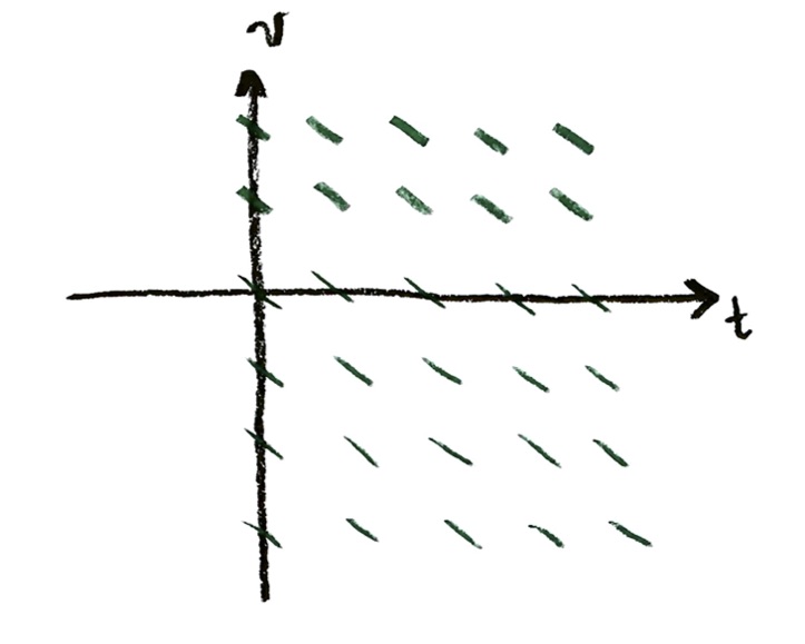
$\dfrac{\mathrm{d}v}{\mathrm{d}t}=-g$,
where $g$ is constant. This gives a slope field you have done already (with different variables) in a previous problem:
A solution curve would just be a straight line. If we drop the object, so that the initial velocity is zero, the solution curve would look like:
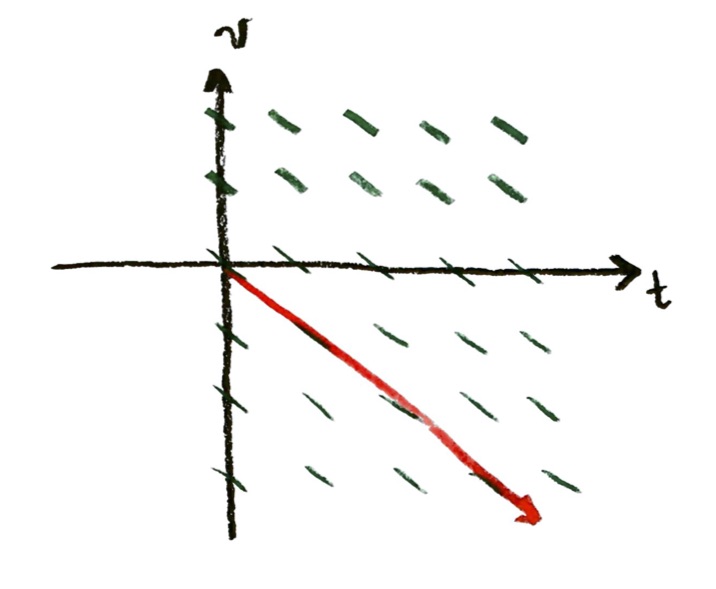
The object has a more and more negative velocity as time goes on. That is, it is moving downwards, faster and faster. Its speed (absolute value of velocity) is increasing linearly with time: the increase in each second is always the same.
This agrees with the explicit solution of the differential equation: if
$\dfrac{\mathrm{d}v}{\mathrm{d}t}=-g$,
then the solution to this is
$v=-gt + C$,
where $C$ could be any constant. In fact, $C=v_0$, the initial velocity at time 0. So for the solution curve we drew, $C=0$, and $v=-gt$. The curve is a straight line, with negative slope $-g$.
Well, what if we don’t ignore air resistance??
Problem: Falling with air resistance
Air resistance is an amazingly complicated phenomenon. There are engineers who spend their whole careers trying to figure out how to minimize or harness wind resistance. But in the spirit of modeling that I said, we can start with the simplest possible assumptions.
For a given object, the most important fact about air resistance is that it gets bigger as the velocity gets bigger. Go faster, you feel more air resistance.
What would be the simplest assumption to make about this relationship? That would be proportionality. That is, we could assume that if there is twice as much velocity, then there is twice as much force from air resistance. Three times the velocity, three times the force. Half the velocity, half the force. In other words, “proportionality” means we are assuming a linear relationship between air resistance and velocity. It’s not exactly true, but it’s actually a pretty good approximation.
What this means as an equation is that
$F_{\text{air}}=-kv$,
for some unknown constant $k$. The $k$ will depend on the size of the object, the exact shape of the object, the texture of its surface, the density of the air, and possibly other things. But we are assuming those are all fixed, so we lump them into a constant $k$.
Note that I am assuming the constant $k$ is a positive number. The minus sign in my equation indicates that, if the velocity is positive, then the force is negative; if the velocity is negative, then the force is positive. The force of air resistance points in the opposite direction to the direction of travel. (Right?)
If we put this into Newton’s law of motion, we get the following differential equation for the velocity as a function of time:
$\dfrac{\mathrm{d}v}{\mathrm{d}t}=-g-\dfrac{k}{m}v$.
Let’s see what this differential equation is predicting!
Problem: Falling object with air resistance
a) Draw the slope field for the differential equation above. Note that, since we don’t have particular numbers for the constants g, k, and m, you will have to draw the slope field qualitatively and conceptually, like I described doing in the last example. Figure out if the slopes will be constant on vertical or on horizontal lines. Then figure out at what points the slope will be zero (equilibrium). Then figure out what happens to the slopes above or below that equilibrium.
b) Draw the solution curve corresponding to dropping the object, so v=0 when t=0.
c) Interpret that solution curve physically. What is happening to the object over time? Does this make sense? (If it doesn’t, you might want to look back at part (a) and check that you did things correctly!)
d) What happens to the velocity after long times, $t\to\infty$? Does this make sense physically?
e) Draw some other solution curves. There should be three “types” of solution curves, similar to the last example that I did above.
c) Figure out what each of these solution curves would mean physically, in terms of the initial condition. What happens over time, physically, in each case? Do these predictions make sense physically?
Problem: Newton’s law of cooling
Let’s do another modeling example.
Here’s the thing I want to model: a hot object that is cooling down. Or, a cold object that is heating up.
Let’s say the temperature of the object is $T$. The temperature $T$ depends on time $t$. Let’s say that the room temperature is fixed; let’s call the room temperature $R$, which we assume to be constant.
Let’s assume that the object cools down or heats up continuously.
It is observed that very hot objects cool down faster than objects which are less hot (less above room temperature). Similarly, very cold objects heat up faster than objects closer to room temperature.
Newton made the following assumption to model this situation:
the temperature changes with time at a rate which is proportional to the difference between its temperature and the room temperature.
This isn’t 100% true, but like I was saying before about population models, it’s a good to start with the simplest reasonable assumption, and see how far that gets you.
Note that “proportional” means “equal to a constant times”. If $A$ and $B$ are “proportional”, then their ratio A/B is a constant, A/B=k, so that A=kB for some constant k.
Problem: Newton’s law of cooling
a) Set up a differential equation for the temperature $T$ as a function of time $t$, which expresses Newton’s assumption above. Your answer will involve the room temperature $R$, and you’ll also need to introduce a proportionality constant (which you can call whatever you like).
b) Draw the slope field for this differential equation. (Because you don’t have specific numbers for the room temperature and the proportionality constant, you’ll have to draw the slope field qualitatively and conceptually, like I described in a previous example.)
c) Draw some solution curves for this slope field. There should be three basic “types” of solution curves (like in a previous example I did).
d) Check the predictions physically: the solution curves are supposed to describe the temperature of a cooling (or warming up) object as a function of time. Do they make sense physically? Do they work in all three cases? If so, great, explain why they make sense to you! If not, though, take a look back at your differential equation, and see what you might have gotten incorrect, that would give you these wrong predictions.
Refining the population model
Let’s go back to the population model that I described in the previous lecture. As the name “exponential growth model” suggests, this predicts an explosive growth of the population.
This is pretty accurate for situations for limited times, where death is not important, and where resources are plentiful. For example, in cell biology, when you have some cells in a growth medium on a dish, the cells happily have plenty of space and food. If you are growing the cells for a few hours or days, people commonly use the exponential growth model to predict how many cells will be present at a given time. It works pretty well.
But, if you extrapolate that equation to longer times, you find that the equation is predicting that after some weeks or months, there will be so many cells that they fill the whole lab, the whole campus, the whole world. We’ve exceeded the range of validity of the model!
If you recall, we vastly oversimplified. In particular, we ignored any limitation on resources: we assumed the organisms could happily reproduce at a constant percentage rate, forever. If we run the equation for long enough, that’s not very realistic.
Presumably, as resources start to reach their limits, that reproduction rate $r$ cannot any longer be constant; it must depend on the population $P$. For a small population, it is the same $r$ that we assumed before; but for larger populations that are reaching the limits of food and space, the $r$ must become lower. So $r$ must not be a constant, but rather a function of population $P$. (Or, at least, that is one way to look at the question of limited resources.)
Open-ended problem: Population growth with limited resources
Here’s an open-ended problem to try out. See if you can make a guess about how $r$ should depend on $P$, to model the assumption of limited food and space. Try to keep things as simple as you can: what is the very simplest mathematical assumption that will reflect our practical assumptions about how $r$ should depend on $P$? Once you have a guess for this dependence, write the corresponding differential equation. Try to draw the slope field, and see what your differential equation is predicting about the population. See if that makes sense! If it doesn’t, go back to your model assumptions, and see if you can correct them in a way that gives predictions that are at least plausible.
What next?
There are two directions I want to go after this.
First, I want to explain how to find explicit solutions for some of these differential equations. That is, I want to find an actual formula for the solution curves that we have been drawing just visually. We’ve seen how to find explicit solutions for very simple differential equations, like dy/dx=1, or dy/dx=x, but that’s it so far. This is a very big question (there’s a whole course on it next term!), but I want to at least show how to solve some of the other simple differential equations. This process will involve natural exponential and logarithm functions, and I’ll re-define and explain these for you, as well as tell you some new things about them.
Second, I want to continue this for differential equations that have more than one variable depending on time. For example, I might have population equations for a prey and a predator species, each of which population depends on time (and on the population of the other). Or I might have a disease model, that models number of susceptible people and number of infectious people. In physics, I have both velocity and position depending on time, and their rates of change might depend on each other. This will lead to something called “phase plane analysis”. It will also lead us back to trigonometric functions, and ultimately back to the Kepler problem where I started the term.