In this lecture, I want to introduce how differential equation models are created and interpreted. In the process, I’ll talk about the geometrical meaning of the derivative, and introduce the concepts of slope fields and phase planes. As well as being useful in itself, this will lead into exponential and logarithmic functions, and from there will lead back to trigonometric functions and ultimately the Kepler problem again!
I know that things have been pretty physics-y so far. So, although there are many physics examples I could give here, I’m going to do some examples from different fields for a bit.
Example: simple population growth
Let’s start with modeling population growth. These could come up in biology (e.g. growing a culture of cells), ecology (a population of animals), or geography/economics (a population of people).
There are many complicated factors to take into account when thinking about population growth. We might want to consider:
- how quickly does the organism reproduce?
- how does the organism reproduce? (do individuals need to find mates? How long do they need between reproductions? Do they need a certain amount of resources? Is it seasonal or continuous through time?)
- are the resources (like food and space) limited?
- is there disease? Are there predators, war, competition?
You could probably add many things to the list. It’s tempting to try to put as many things as we can into the model, to make it more realistic.
However, one counter-intuitive principle of modeling is that this is NOT a good place to start. There are a number of problems with trying to put too many factors into the model to begin with:
- it’s hard to know where to start, and we’ll get confused
- if the model is too complicated, there will be too many parameters to try to estimate when comparing to reality
- it will not be clear what the most important factors are when comparing to reality, so we won’t get any insight into the actual dynamics driving the observed behavior
- a model with two many parameters actually starts to lose predictive power, because it can start to fit anything
Contrary to what you might think, usually the best place to start when creating a mathematical model is to strip things down as much as possible. We want to idealize to the point where it seems almost too simple. If we can isolate just one factor of the thing we are trying to model, then we have a chance of writing a reasonable equation that describes that factor. Then, we can see what the model predicts. Sometimes, just one very simple factor will do a surprisingly good job! But sometimes, that model will prove to be TOO simplified. But that’s OK: it will be easier to add things to our simple model, slowly and one at a time, rather than start with something that is too complicated and trying to pare it down.
Let’s see how this looks for population growth. I’m going to make things as simple as possible:
- let’s only focus on growth. So I’m going to ignore predators, disease, war.
- in fact, I’m going to ignore death! Let’s say the organisms are immortal. (Or, at least, that they live longer than the time period I’m concerned with.) Not so realistic, but remember, we are paring down as much as we can.
- Let me also ignore problems of gestation period, finding mates, etc. So, I could imagine that I have something like binary fission of single-celled organisms. The model will also work to model more complicated things like mammals, but it’s going to leave out the more complicated features of reproduction; depending on what we’re interested in, that may be an oversimplification, but let’s start simple now and add complications only as needed.
OK, so what am I left with? I’m going to leave in the growth rate: so I have only one factor or dynamic that I’m modeling, how the population grows.
Now, are we talking about absolute growth rate (number of new individuals per unit time), or about relative growth rate (some proportion of our population of individuals will reproduce per unit time)?
Assuming an absolute growth rate would mean that our population grows linearly, the same number of new individuals each hour or year or whatever our time period is. That’s a little TOO simple: as we have more individuals, we have more individuals to reproduce. THAT is the core dynamic that I’m trying to describe.
So, let’s assume that the relative growth rate is constant. That is, in each time period, some percentage of the individuals will create a new individual. The period might be one year (if we’re talking about squirrels) or one hour (if we’re talking about yeast). The rate will depend on the organism. Let’s say, for argument’s sake, that the rate is 10%: each time period, 10% of our individuals will create a new individual. Then if we have 1000 individuals at the start, we will have:
| Time | Individuals | New individuals created |
| 0 | 1000 | 1000(0.10)=100 |
| 1 | 1100 | 1100(0.10)=110 |
| 2 | 1210 | 1210(0.10)=121 |
| 3 | 1331 | 1331(0.10)=133.1 |
| 4 | 1464 | 1464(0.10)=146.4 |
Such a model is called a difference equation. We can write it out as an equation: in each time period, our population increases by $\Delta P$ individuals. The number of new individuals created is equal to 10% of the current population. Therefore,
$\Delta P = (0.10) P$,
where $P$ is a variable that depends on time $t$ (that is, it is a function of $t$), and the $\Delta P$ is understood to be for one time period.
If the rate was some other number, rather that (0.10), we could just put that number $r$ in place of the (0.10) in the equation:
$\Delta P = r P$,
where $r$ is a constant, to be determined from observation.
This gives us a model for the growth! We can measure the growth of our cell culture, say, for a few time periods to estimate the rate $r$. Then we can make a table like the above.
There is a lot more to say about difference equations, where the time step is discrete. But I’m going to not do them justice in this class, because I want to focus on differential equations, where we make the change continuous.
Differential equations versus difference equations
Now, let’s imagine that our organisms are always reproducing. (They’re not like squirrels, with a breeding season; they’re more like yeast.) Then the table we wrote above is a little bit not representative: during that first time interval (first day or hour or whatever), the organisms are growing. There are some new organisms produced during that first time interval which we aren’t accounting for. That won’t be a big deal if the time interval is relatively short, compared to the rate of growth of the organisms; but if the time interval is on the long side, we should take this into account.
That is, if we again assume that 10% of individuals are, on average, reproducing per growth period, then 5% of them should reproduce in the first half of a time period (assuming that the times they reproduce are randomly distributed). That is, 5% is 0.5 of the 10% rate, because we are looking at 0.5 of a time interval. If we start with 1000 individuals, then after half a time period we should have 1050; then, in the next half-period, those 50 individuals are also reproducing, so after one time period, we would have 1103. Our table would look like:
| Time | Individuals | New individuals created |
| 0 | 1000 | 1000(0.10)(0.5)=50 |
| 0.5 | 1050 | 1050(0.10)(0.5)=52.5 |
| 1.0 | 1102.5 | 1102.5(0.10)(0.5)=55.1 |
| 1.5 | 1157.6 | 1157.6(0.10)(0.5)=57.9 |
| 2.0 | 1215.5 | 1215.5(0.10)(0.5)=60.8 |
| 2.5 | 1276.3 | 1276.3(0.10)(0.5)=63.8 |
| 3.0 | 1340.1 | 1340.1(0.10)(0.5)=67.0 |
Note that I’ve started keeping decimals. I’m idealizing more here: I’m keeping decimals when I do the calculations, then I’ll round off to a whole number of individuals in the final answer if needed. Note also that it doesn’t make a huge difference, but that’s because of my numbers: with other numbers (like if $r$ was larger), the difference would be bigger. And even in this case, the differences will start to get substantial if I run this for longer times.
But why stop at half time periods? During that first half a time period, the organisms were reproducing as well. So, in the first (0.25) of a time period, we would have (10%)(0.25)=2.5% of the organisms reproducing. And those extra 2.5% would have a chance to reproduce in the following (0.25) of a time period. So our table would look more like
| Time | Individuals | New individuals created |
| 0 | 1000 | 1000(0.10)(0.25)=25 |
| 0.25 | 1025 | 1025(0.10)(0.25)=25.63 |
| 0.50 | 1050.63 | 1050.63(0.10)(0.25)=26.27 |
| 0.75 | 1076.90 | 1076.90(0.10)(0.25)=26.92 |
| 1.00 | 1103.82 | 1103.82(0.10)(0.25)=27.60 |
And why stop there? In every 0.1 time periods, we would have 10%(0.1)=(0.10)(0.1)=0.01=1% of the organisms reproducing, and they would go on to reproduce in the next 0.1 of a time period . . .
| Time | Individuals | New individuals created |
| 0 | 1000 | 1000(0.10)(0.1)=10 |
| 0.10 | 1010 | 1010(0.10)(0.1)=10.10 |
| 0.20 | 1020.10 | 1020.10(0.10)(0.1)=10.20 |
| 0.30 | 1030.30 | 1030.30(0.10)(0.1)=10.30 |
If $\Delta t$ is the fraction of a time period that we are looking at (like, 0.5 of a time interval, or 0.1 of a time interval), then the percentage of individuals that reproduce is $(0.10)\Delta t$. (Right? Check that with what I wrote above.) So the number of new individuals $\Delta P$ that are produced in that fraction $\Delta t$ of a time interval are
$\Delta P=(0.10)(\Delta t)P$,
which I’ll usually write as
$\Delta P=(0.10)P(\Delta t)$.
That’s still a difference equation, but for the shorter time interval $\Delta t$. If I want to imagine the organisms continuously growing, then I would take the limit as the $\Delta t$ gets smaller and smaller. For an “infinitely small” time period $\mathrm{d} t$, the infinitesimal increase in the population will be $\mathrm{d} P$, given by
$\mathrm{d} P = (0.10) P \,\mathrm{d} t$.
This is called a differential equation, because it is an equation for the differentials! This differential equation models the continuous growth of a population, at a continuous rate of 10% of individuals, on average, reproducing per time period. (Which does not mean the population will actually grow 10% in one time period! It will grow more, for the reasons I talked about just above.)
This differential equation can also be seen as an equation for the derivative, because we can rewrite it as
$\dfrac{\mathrm{d}P}{\mathrm{d}t}=(0.10)P$.
The population $P$ is an unknown function of time, which we’d like to figure out. What we know, from the assumptions of our model, is something about the derivative of this unknown function! So the calculus difficulty will be to find the function, knowing something about its derivative!
If the rate was some value $r$, instead of 10%, then these equations would become
$\mathrm{d} P = r P\, \mathrm{d} t$
or
$\dfrac{\mathrm{d}P}{\mathrm{d}t}=rP$.
This lovely differential equation goes by the name exponential growth model (and we’ll see the reason for the name in due time!).
But wait, is this really realistic?
You may have been saying to yourself, but wait! Does this actually make sense?
That is a very reasonable worry! Even yeast are not really growing continuously: they can only grow one yeast cell at a time. And fractional individuals don’t really make sense in the real world. And, besides, looking at my tables, number-wise it didn’t seem to make all THAT much difference. So why am I insisting on continuous growth?
One answer is that continuous growth is often a good approximation, when the number of individuals is large. If we are talking about millions of yeast cells, or about the human population of the world, the numbers are so big that it is a good approximation to imagine the number changing continuously. Also, with large numbers like that, the assumption of continuous growth makes a bigger difference.
Another answer is that I will also want to model different kinds of growth or decay, where the numbers are large and so continuous growth is a good model.
However, some populations really make more sense as difference equations. If we have a small number of individuals, or if we have a discrete breeding season, then continuity is not a good assumption. So why focus on continuity?
Surprisingly, it’s often easier to understand a differential equation (with continuous change), than it is to understand a similar difference equation (with discrete changes). So even when we want to model a system with discrete changes, people often start off by modeling with differential equations, which are easier to mathematically understand!
Actually, this really misled people for a long time. People would make a differential equation model for something (like a population), and assume that the difference equation model wouldn’t behave too differently. In fact, once computers came around (which could compute difference equation models very quickly), people started to realize, with great surprise, that the difference equation might behave VERY differently from the differential equation! This was first noticed by a biologist, Robert May, in 1976, when we was studying population models much like the ones we will be doing soon. This was one of the starting points of the theory of “chaos” and dynamical systems.
If you want to learn more about difference equations (and about modeling), you should take Katie’s class, Quantitative Reasoning and Mathematical Modeling. Katie’s expertise is in modeling, and in chaos and dynamical systems. In this class, we are going to concentrate on models with continuous change, so differential equations.
How to read a differential equation
Let’s look at the differential equation that we developed to model population growth (the “exponential growth equation”). It was
$\mathrm{d} P = r P \mathrm{d} t$
or
$\dfrac{\mathrm{d}P}{\mathrm{d}t}=rP$.
The first equation is saying that, in a short time period $\mathrm{d} t$, the population is changing by an amount $\mathrm{d} P$. That change in population is proportional to the population itself; the proportionality constant is $r$.
The second equation is saying that the (absolute) rate of change of the population with time, $\frac{\mathrm{d}P}{\mathrm{d}t}$, is equal to the population times a rate constant $r$. Bigger population, bigger absolute growth rate, in an entirely proportional way. Twice the population, twice the absolute rate of growth (because twice as many individuals to be reproducing). Ten times the population, ten times the absolute rate of growth.
Very often, a scientific paper will show you their differential equation model for something, and an important skill is to read through what it is claiming conceptually.
The differential equation model encapsulates our assumptions about the mechanics of the system. All the practical things we said at the beginning—about there being no disease, no limits on resources, no complicated breeding—are all reflected in the simple model we created.
What is a “solution” to a differential equation?
The “solution” to the differential equation
$\dfrac{\mathrm{d}P}{\mathrm{d}t}=rP$
would be a function $P$, depending on time $t$, which would obey that condition. In other words, the “solution” would be a formula that gives the population $P$. The formula would involve $t$, and it would have the property that if you took its derivative, you would get the same formula again, just multiplied by $r$.
Practically, the differential equation tells you how the population changes from one time moment to the next. To “solve” the differential equation is to figure out what the population is going to be in one year, ten years, one hundred years.
I can’t show you a solution of this differential equation yet, because we still need to figure it out. But let me give another example: let’s say our differential equation was
$\dfrac{\mathrm{d}P}{\mathrm{d}t}=(0.10)t$.
Then a solution of this equation would be $P=(0.05)t^2$, because if you take dP/dt for this function, you get (0.10)t, as required. This differential equation has infinitely many solutions: $P=(0.05)t^2+C$, where $C$ can be any constant. The value of the constant is determined by the initial condition; if I know the value of $P$ at time $t=0$, then I can determine $C$.
The exponential growth differential equation
$\dfrac{\mathrm{d}P}{\mathrm{d}t}=rP$
is a trickier beast, because it says that $P$ should be a formula whose derivative equals $r$ times the same formula. We’ll see how to find such a function soon!
We will see some methods for figuring out solutions of differential equations. If you take the Ordinary Differential Equations course next term you will see many more! However, it’s worth noting that frequently, we can NOT find any explicit formula for the solution of a differential equation. That doesn’t mean the solution does not exist; it just means that we can’t give a formula using standard functions that we know. However, that doesn’t mean all hope is lost: in fact, we will be able to figure out a lot about a solution of a given differential equation, without necessarily having a specific formula for it.
What is a differential equation model?
Setting up the differential equation is modeling: that is where our assumptions and knowledge about the real-world system come into play. Finding the solution of the differential equation is purely math: that is applying techniques of calculus. At that point, I forget that this is a real-world problem; I just want a function $P$ that obeys a certain mathematical condition. Of course, once I find that function, then I can make predictions about the real world based on my model, and I can compare them to what I observe in reality. In response to that, I might decide to change my model, perhaps to put in some effect that I left out before.
This back and forth, between creating a model, making mathematical predictions, going back to compare to reality, then refining the model, is the subject of applied mathematics.
If you’d like to know more about the relationship of mathematical models to real observations, I recommend starting by reading this excerpt from a book by Timothy Gowers called Mathematics: A Very Short Introduction.
How to approximately numerically solve a differential equation
A little ironically, if we want to numerically calculate what a differential equation is predicting, the idea is to convert it back to a difference equation. That is, replace the differential equation, for example
$\mathrm{dP}=(0.10)P\,\mathrm{d}t$
with a difference equation
$\Delta P = (0.10) P \Delta t$,
where we take a small value for $\Delta t$. Then we calculate tables, like I did in the example at the beginning. The smaller the $\Delta t$, the better the approximation to the continuous differential equation.
How to picture a derivative
I want to describe how to picture a differential equation. But there’s a problem: I haven’t talked yet in this class about how to picture a derivative! So, first, I want to talk about how to picture a derivative. Then, I want to apply that to picture a differential equation.
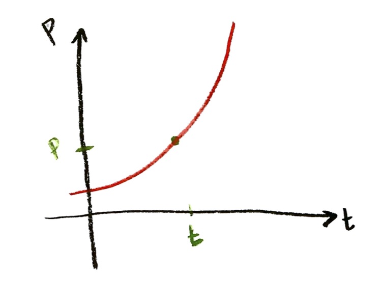
Let’s suppose that $P$ is a function of $t$. And let’s suppose we draw a graph of this function; say it looks like this:

Now, let’s pick some specific value $t$ for the time. The meaning of the graph is, if I go over $t$ units from the origin on the horizontal axis, then I go up to the graph, then the height of that point gives me the value $P$ of the population, at that value $t$ of the time:
Now, suppose we increase the time slightly. That is, we choose another time $t+\mathrm{d}t$, which is $\mathrm{d}t$ larger than $t$. This slightly later time will correspond to a slightly larger population, $P+\mathrm{d}P$. This looks like:
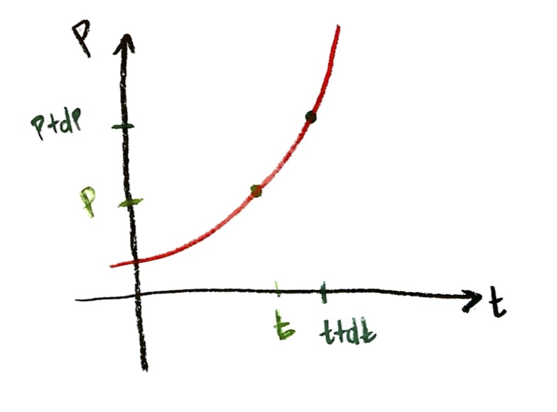
Now, compare the positions of those two points on the graph. Compared to the first point, the second point is moved over $\mathrm{d}t$ time units horizontally, and is moved up $\mathrm{d}P$ population units vertically:
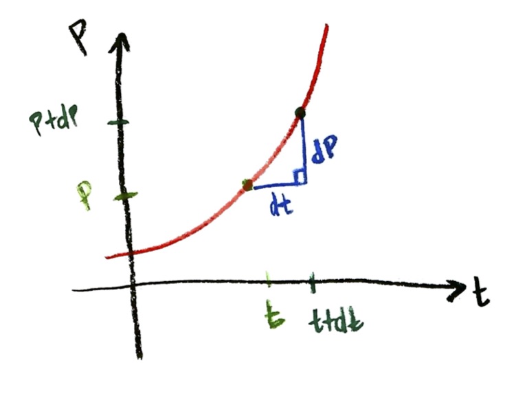
You may recall from high school that the ratio of “up/over”, or “rise/run”, is referred to as the slope of the straight line between the two points. So, the ratio
$\dfrac{\mathrm{d}P}{\mathrm{d}t}$,
which is the derivative of $P$ with respect to $t$, on the graph represents the slope of that little red line segment!
But wait: that little red line segment isn’t a straight line! That’s why we have to take the $\mathrm{d} t$ to be very small: it is assumed small enough that we can approximate the segment of the curve as a straight line. Alternately, we can say that we are zooming in to the curve closely enough that it resembles a straight line. Alternately, we can say that we are taking the limiting value of the slope, as we take the $\Delta t$ smaller and smaller.
All this boils down to:
the value of the derivative $\dfrac{\mathrm{d}P}{\mathrm{d}t}$ at some $t$ gives the slope of the graph of $P$ versus $t$, at that value of $t$.
That “fact” is a little bit circular: in mathematics before calculus, you only define “slope” for straight lines. So this “fact” is really kind of a definition: this is what we mean by the slope of a curved line! To find the slope of a curve at some point $(t,P)$, we find another point $(t+\mathrm{d}t,P+\mathrm{d}P)$ on the curve really nearby, and find the slope between those two points.
If you’d like more explanation of this, I strongly recommend reading Chapter X: Geometrical Meaning of Differentiation, in the book Calculus Made Easy by Silvanus Thompson. (The chapter starts on page 97 of the pdf.)
Note that $\frac{\mathrm{d}P}{\mathrm{d}t}$ is also, practically, the rate of change: it says at what absolute rate $P$ changes with respect to time $t$. In our population example, its units would be individuals per unit time. So, if the graph has a large slope, it means the population is increasing rapidly; a small slope means increasing slowly; a negative slope means the population is decreasing.
Note that the absolute rate of change of population with time will be changing over time. In our exponential growth model, it’s going to be growing slowly at first, (small slope), and then faster and faster over time, (bigger slope), as the population gets bigger and there are more and more individuals to be reproducing.
How to picture a differential equation
OK, so this section was about differential equations. How do we picture a differential equation, for example,
$\dfrac{\mathrm{d}P}{\mathrm{d}t}=(0.10)P$?
The problem is that we don’t yet know what the curve $P$ as a function of $t$ looks like. That would be the “solution” to this differential equation.
The differential equation is not telling us what the population is at any given time. But what it IS telling us is, IF we knew the population, THEN it tells us the SLOPE of that graph.
Let me give a numerical example. Suppose the time $t=0$, and the population $P=1000$. Then the differential equation tells me that
$\dfrac{\mathrm{d}P}{\mathrm{d}t}=(0.10)(1000)=100$.
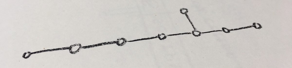
This means that, IF the curve goes through the point $(t,P)=(0,1000)$, then its slope there is $100$. Let me draw this:
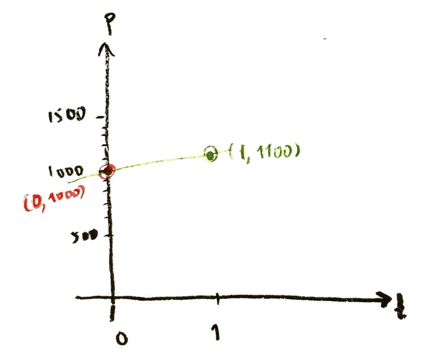
See what I did there? I drew the point (0,1000). Then I knew that, IF the graph goes through that point, it must have slope 100. So I drew a line from (0,1000) to (1,1100), which would have slope 100.
But wait! As we discussed before, the graph wouldn’t keep having that same slope, all the way from time $t=0$ to time $t=1$. The slope would actually increase. All I know is that the slope RIGHT AT (0,1000) is equal to 100. So, I should draw my little slope line smaller, just at the point (0,1000):
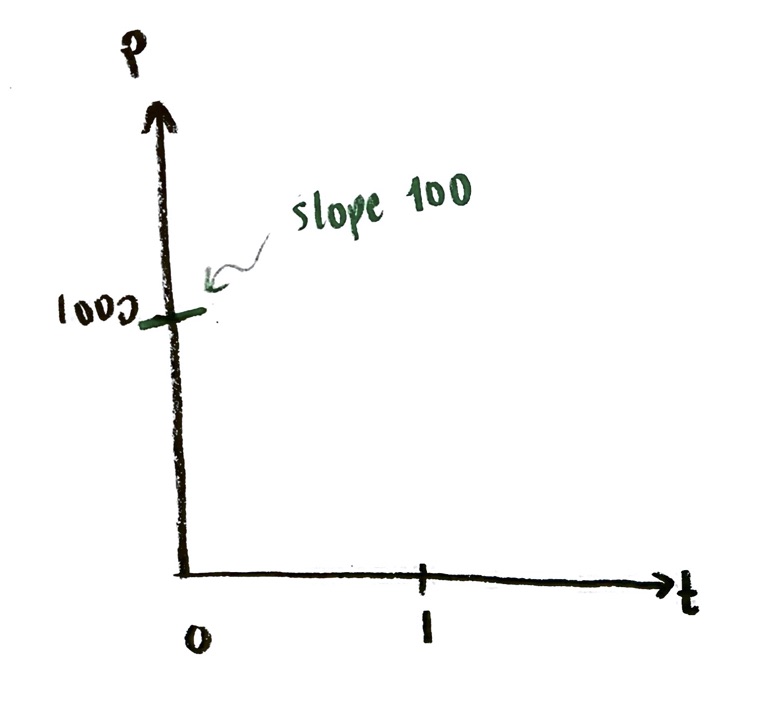
Of course, if I drew the slope JUST at that point, the line would be invisible! So I have to make the slope line big enough to see. But the assumption is that the little green line is just giving the slope of the curve AT the point (0,1000). And that’s only IF the curve does in fact go through the point (0,1000), which we don’t know!
Now, it’s hard to see the exact value of the slope just from drawing a little line segment. So we aren’t going to try to make this exact. Instead, we are looking for a qualitative picture of what the slopes are. Let’s zoom out a little:
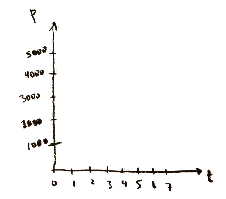
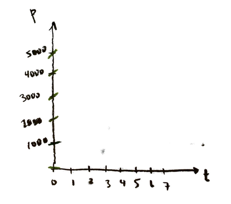
Now, let’s figure out the slope at some more points. I’m going to start by figuring out slopes at some representative points on the vertical P axis:
| Point | Slope |
| (t,P)=(0,0) | dP/dt=(0.10)P=(0.10)(0)=0 |
| (t,P)=(0,1000) | dP/dt=(0.10)P=(0.10)(1000)=100 |
| (t,P)=(0,2000) | dP/dt=(0.10)P=(0.10)(2000)=200 |
| (t,P)=(0,3000) | dP/dt=(0.10)P=(0.10)(3000)=300 |
| (t,P)=(0,4000) | dP/dt=(0.10)P=(0.10)(4000)=400 |
| (t,P)=(0,5000) | dP/dt=(0.10)P=(0.10)(5000)=500 |
The important thing here is that the slopes are increasing as P increases. So I can draw that on my graph, at least qualitatively:
I don’t know if I’ve really succeeded at drawing a line of slope exactly 500 at the point (0,5000). But the point is that I have drawn the lines getting more and more sloped, as we move up the P axis.
Note that I don’t know where the function of P versus t hits the P axis. In practical terms, I haven’t been given the initial population at time $t=0$. That is not part of the differential equation; it’s called an initial condition, and it’s a separate piece of data that I’m not assuming I have yet.
Now, I’ve only done points with time $t=0$. So let’s do some points with other values of t. Let’s say $t=1$. Then we have:
| Point | Slope |
| (t,P)=(1,0) | dP/dt=(0.10)P=(0.10)(0)=0 |
| (t,P)=(1,1000) | dP/dt=(0.10)P=(0.10)(1000)=100 |
| (t,P)=(1,2000) | dP/dt=(0.10)P=(0.10)(2000)=200 |
| (t,P)=(1,3000) | dP/dt=(0.10)P=(0.10)(3000)=300 |
| (t,P)=(1,4000) | dP/dt=(0.10)P=(0.10)(4000)=400 |
| (t,P)=(1,5000) | dP/dt=(0.10)P=(0.10)(5000)=500 |
It’s the same thing!! Why? Because there is no $t$ in my formula for slope! The slope dP/dt is given by (0.10)P. This particular differential equation doesn’t involve the $t$ in the formula for the slope. So the slope is independent of t. (Such a differential equation is called autonomous.)
That means the slopes at the points (0,1000), (1,1000), (2,1000), (3,1000), . . . are all the same! So I can draw some little slope lines in at those points too, pretty easily:
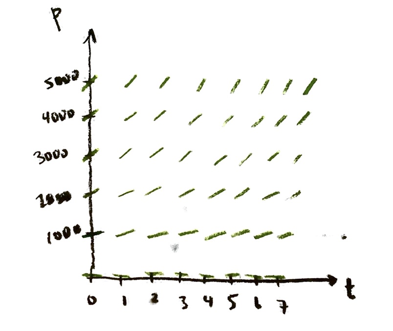
I haven’t done a perfect job here. But what I’m trying to show is that the slope is constant on horizontal lines, equals zero on the t-axis, and gets larger as we go up vertically.
Negative values of t and P don’t make much sense in our model. But it can be sometimes helpful to mathematically understand the equation to allow for negative values as well. Negative values of t don’t change much: the slopes are constant in t. For negative values of P, the slope is negative (right?). So we get a picture like:
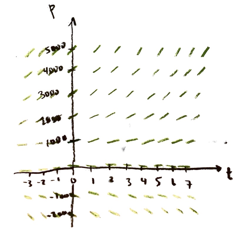
Note that, really, there should be a little slope line attached to EVERY point (t,P) in the t-P plane. We have no idea where the graph of P versus t goes through yet; it could go through a point like (0.5, 1300), so theoretically I’d have to imagine a little slope line attached to that point (of slope 130). But if I try to draw ALL the slope lines, (a) it will take me a very long time, and (b) I’ll just end up with an unreadable plot, totally filled with green lines. So, I just pick a representative grid of points.
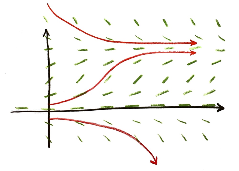
This picture is called a slope field. It is a picture of the differential equation dP/dt=(0.10)P. It represents the condition that, at whatever point (t,P) the solution curve goes through, its slope there must be given by (0.10)P.
Practically, this reflects the fact that the differential equation never tells you what the population IS. It tells you, IF you know the population at a certain moment, how the population will CHANGE in the next moment. That is, it gives you the small dP, if you set a small dt. But only for small dt: it only gives you the next little step. Because once you move by dt in time, the population changes to P+dP, and now you have to recalculate the slope based on the new population.
How to picture solution curves to the differential equation
Once we draw the slope field to a differential equation, we can get a pretty good qualitative sense of what a solution curve will look like.
There is more than one possible solution curve. In fact, there are infinitely many. The solution curve depends on the initial condition. Once we choose a starting point in the slope field, then the slope field tells us what the rest of the curve has to look like.
For example, if I take the starting condition of P=1000 at the initial time t=0, then I will get a solution curve that roughly looks like

I am trying to make the red curve have slope equal to the slope field at all of its points. Again, you have to imagine that there are lots of little green lines, inbetween the ones I drew: the slope field exists at every point. At each of those points, if I find the slope dP/dt of the curve (by zooming in really close on two points close together), that slope should agree with the slope field.
If I choose a different initial condition, I will get a different curve following the slope field:
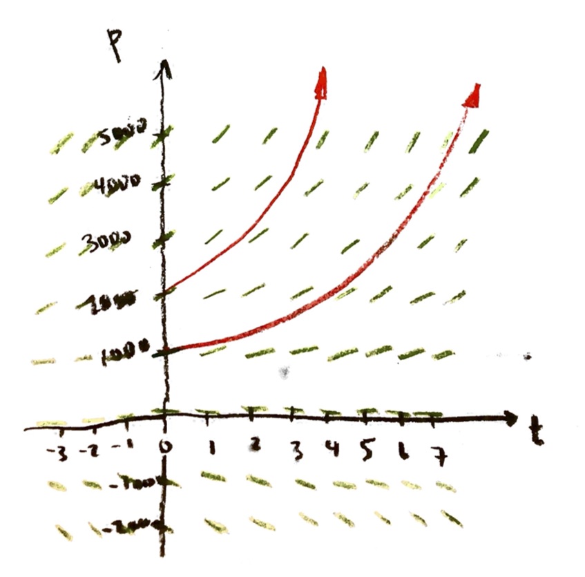
If I keep picking different initial conditions, I get a whole family of solution curves, one for each initial condition.
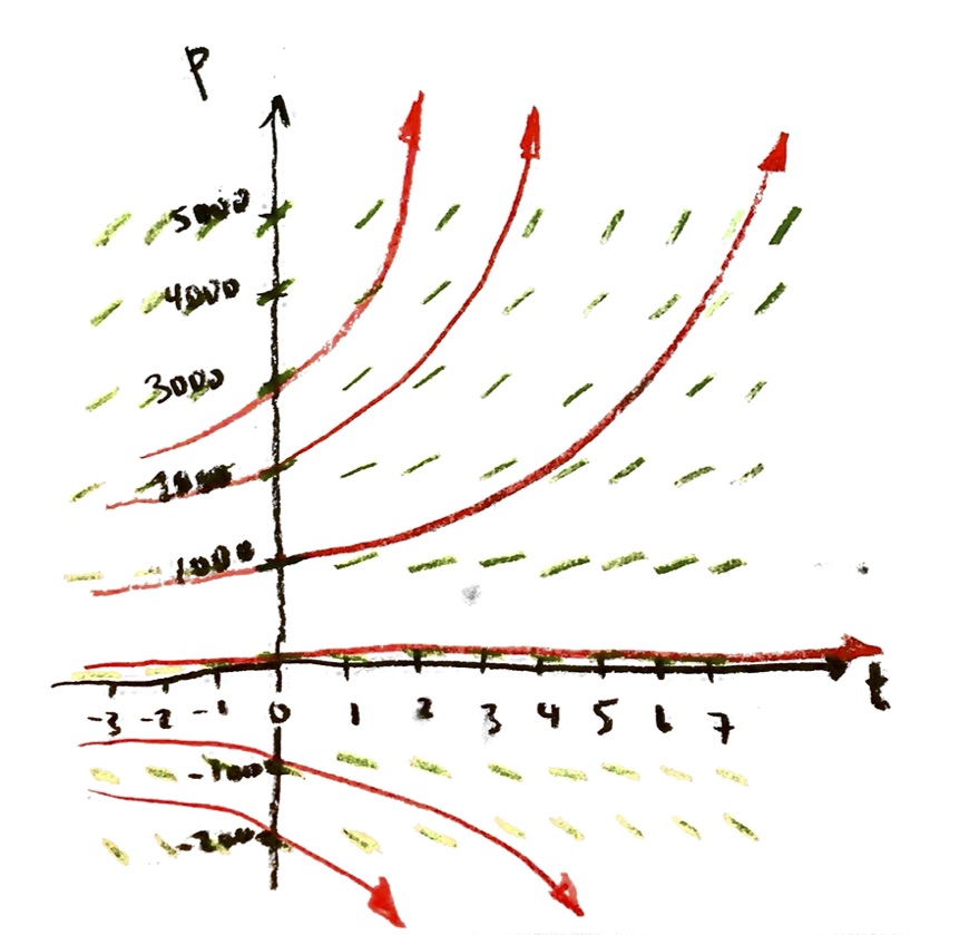
Again, in principle, I have infinitely many solution curves; but if I tried to draw them all, it would get very messy.
In summary:
- The differential equation tells you what slope the unknown solution function should have at every point. It therefore gives you a slope field.
- Picking an initial condition picks out one particular solution of the differential equation. Graphically, you start at that point, and then make a curve which follows the direction of the slope field at each point.
- These graphical solution curves represent solutions of the differential equation. A solution of the differential equation is a function which satisfies the condition that the differential equation is saying.
Where next?
Phew, I’m tired! That was a lot.
In the next lectures, I’m planning to do (or get you to do) three things:
- Set up more differential equation models, based on different real-life situations.
- For different differential equations, draw the slope fields and typical solution curves, and use that to make predictions about the behavior of the system.
- For some simple differential equations, (including the exponential growth equation), to show how to find explicit formulas for the solutions, based on ideas we have developed so far.