Category: Logarithms

Hmm, my titles are getting longer.

In this lecture, I want to take a different viewpoint on the definition and purpose of logarithms. In this point of view, the point of a logarithm is that it is the inverse operation of taking a power. (That statement isn’t exactly right—I’ll fix it as we go along—but that is the general idea.)

The “practical” part of my title means that I’ll focus on how this allows you to work with and solve equations involving powers. Later (if I don’t get exhausted first), I’ll come back and look at inverse operations a little more theoretically.

This version is the most common introduction to logarithms nowadays. If you did logs in high school, this is the version you most likely saw.

Inverting exponentials

So, how does this work? Let me go back to the counting zeroes. If we say that, for example, log(1,000) = 3, we are saying that 1,000 has 3 zeroes. Stated differently, : the number 1,000 consists of 3 factors of 10. That is:

log(1,000) = 3 means .

The logic is reversible:

means log(1,000) = 3.

As we’ve seen, we can extend this logic to numbers that are not whole. For example, means , and means . Or, doing things exactly:

means , and

means .

So, for any positive number x,

log (x) = y means .

(Reread this, comparing it to the numerical examples above, and make up some more numerical examples, until you feel confident you understand it. It’s easy to get the x and y mixed up here.)

The logic is reversible:

means log (x) = y.

Usually in this second version, people tend to switch the x and y, because the habit is to think of x as the input of a function, and y as the output.

So, to summarize: for any positive number x:

y= log (x) means ;      (1)

and, for any number x:

means x = log (y)      (2)

We can state these principles in a slightly different way. In principle (1), if y=log(x) means that , then I can just substitute y = log x into . That means, for any positive number x:

      (3)

Similarly, I can rewrite principle (2) to say, for any number x,

      (4)

Think about what those mean for a moment. In (3), let’s take x = 1,000. Then (3) is saying . For any number x, the number log(x) is “how many zeroes are in x”; then doing is making a number with exactly that many zeroes, which is just x!

Problem 1: Think through principle (4) in the same way.

Principles (1) and (2) say that the functions and are inverse functions; we get one by switching the inputs and outputs of the other. Principles (3) and (4) say that the operations of taking the log(something) and of taking 10^(something) are inverses of each other; they cancel each other out.

In most introductory textbooks I have seen, the book uses principles (1) and (2). I prefer principles (3) and (4), for reasons you’ll see below. They are completely logically equivalent, just a slightly different way of writing and thinking about them.

Different logical orderings

I have started with my idea of “counting the zeroes”; I derived the multiplication principle from that:

log(a x b) = log a + log b      (M)

Then, from (M), I derived rules for division and for exponents:

      (D)

      (E)

Then, in this section, I derived the inverse principles, (1), (2), (3), and (4). (I haven’t really proved everything precisely, but it is possible to do so.)

One can do this in different orders. In Version 3 that we are doing here (which is the usual high school approach), I would start by assuming principles (1) and (2) as defining the logarithm. Then I would derive (3) and (4), and I would derive (M), (D), and (E) as consequences of (1) and (2). Finally, I would interpret the logarithm as “counting the zeroes”.

(I’m not being 100 per cent precise here. For example, I never gave a strict mathematical definition of “counting the zeroes”. And I need to make some assumptions about exponentiation. But it is possible to make all this totally precise, along the lines I’m describing.)

Which thing you start with is a matter of taste and of pedagogical strategy.

Wherever you choose to start, though, it is helpful to be able to switch between the different perspectives on logs, depending on what you are using them for. There isn’t one version that is objectively better than the others.

Solving equations

This version of logarithms is particularly helpful in solving equations that involve exponents.

Example: Let’s say we know that t is a number such that

.

I want to solve this equation for t. (Equations like this come up a lot in applications. I’ll give examples in the next lecture.) What I do is take log of both sides (since the two sides are equal numbers, their logs must also be equal):

   (by (M))

   (by (4))

   (subtracting log(3) from both sides)

   (multiplying both sides by 3.55)

   (I’m estimating in my head, you can use a calculator for more accuracy)

Another example: Note that the power doesn’t have to be of 10 for this to work, because we can alway use property (E), no matter what the base is. Let’s say we know

,

and we want to solve for t. We could use logs base 2 here, but base 10 logs work just as well. (Either base 10 or base e logs are preferable, because those are the ones on the calculator.) Proceeding as before:

   (taking logs of both sides)

   (by (M))

   (by (4)),

and from there it goes very similarly to before. (You should find .)

Problem 2: Solve the equation for the unknown x.

Problem 3: Solve the equation for the unknown t.

Problem 4: Suppose that , , and are some known quantities. Suppose we know the equation holds. Solve this equation for t. (Your answer should be a formula for t, which will depend on , , and . This equation comes up in applications.)

If we have equations where we need to get the variable out of a log, we can solve them in an opposite way, by taking of both sides.

Example: Suppose that we know . I want to solve this for the unknown x. I start by using regular algebra to solve for the log x:

and then I take of both sides:

,

that is,

.

Finally, using (3), I can conclude that .

Problem 5: Suppose that , , and are known numbers, and suppose we know that the equation is true. Solve this equation for the unknown x. (Your answer should be a formula for x, which involves the , , and .)

Graphs

I am now in a position to be more precise about what I said about graphs earlier. Let’s say we have an exponential function. I’ll start with an easy one, then make it more complicated.

Let’s say we the equation . Now, instead of graphing y, I am going to graph the values of . Let’s give this new variable a name; say . Taking logs of both sides of , I get

     (by (E))

,   where z stands for log y, and m stands for log 2.

This means, when I start with , and I instead graph log y versus x, I get a straight line, going through the origin, with slope 2.

In applications, we are often using different letters, so don’t let that throw you off. For example, suppose we start with 1 cell, and that cells divide once every hour. Then, after t hours, the number N of cells we have is

.

Taking logs of both sides, and simplifying as before, we find

.

This means that, if we graph t on the horizontal axis, and log N on the vertical axis, we get a straight line, going through the origin, with slope log 2.

Problem 6: Suppose we have the function , where a, b, and c are some constants, x is the input, and y is the output. Convert this to an equation for log y as a function of x. Simplify as much as possible. Then, describe what the graph will look like. Be as specific as you can: for example, if it is a straight line, say what its slope and y-intercept will be. (Your answers will be formulas depending on the constants a, b, and c.)

Problem 7: Suppose we have a number of individuals N which depends on time t. The number of individuals is growing exponentially, with a doubling time . We start with individuals, at the initial time .
a. Try to convince yourself that the following equation for is true:

.

(It might help, as you are trying to think it through, to put in specific numbers for , , and .)
b. Transform this equation, to get a formula for log N as a function of time t. (If you picked particular numbers for , , and in the previous part, for this part I would like to revert them back to unspecified constants. So your formula for log N will involve the , , and .)
c. Describe what the graph of log N versus t is going to look like. Be as specific as you can.

Logs of negatives

I have said earlier that, if we take either counting zeroes, or property (M), as our defining property of logs, then it makes perfectly good sense to take the log of a negative number: since (-1)(-1)=1, we have

log((-1)(-1)) = log(1),
so log(-1) + log(-1)=0
so log(-1)=0.

This implies that, for any non-zero number x, log(-x) = log(x), because log(-x) = log ((-1)x) = log(-1) + log x = 0 + log(x) = log(x).

On the other hand, if we take (1) and (2) as our defining property of logs, then logs of negative numbers make no sense at all. Suppose that log(-1) existed. Let’s give it a name, say y = log(-1). Then, by property (1), this would imply

.

If you think about this a bit, this is troubling. The number 10 to a positive whole number can’t give a negative answer. If you raise 10 to a fraction, you are taking roots, and roots by definition are positive. If you raise 10 to a negative power, you are getting a fraction, with a power of 10 in the denominator—still positive. There is no way I can solve this equation for y.

This is why people commonly say that logs of negative numbers are undefined. And this is the standard definition today for log: that log x is only defined for strictly positive numbers x (i.e. x cannot be negative or zero).

(But things change if we allow complex numbers… That allows for logs of negatives, but it gives us a different answer than what I’ve said above. And it gives us a whole other perspective on logs. I probably won’t have time to get to this, but I’ll try to at least give hints and references in the final lectures.)

Sometimes, though, we would like to have our Version 1 of logs: sometimes it makes most sense to follow the reasoning above, and say log(-1) = 0, so log(-x) = log(x) for all non-zero x. It depends what we are using the logs for. If we are in such a situation, we can write that version of the log as

.

The absolute value bars around x have the effect of stripping off any negative sign: if x is negative, then by definition |x| is positive (with the same magnitude), so log|-x|=log|x|, and |x| is positive, so your high school math teacher will not feel troubled by a disturbance in the Force. We’ll see later that log |x| is the right version for calculus applications, for example.

Plans for next lectures

Next time, I’ll give some examples of applications! Now that we can solve equations involving exponentials and logs, I will be able to be more detailed than I could have been earlier.

My plans after that:

• Applications
• Version 3b: Logarithms as inverses of exponentials (abstract approach)
• Version 4: Logarithms as a missing function in calculus (and why e)
• How computers calculate logarithms
• Version 5: The modern math version: logarithms as an “isomorphism”
• Looking forward: infinite series, complex numbers…

I won’t be expecting you to do the problems for these, because we are nearly out of time for this class. (I also don’t know if I’m going to run out of energy before finishing all this! I will do my best.) I would like you to have this material, though, because I think these topics are all interesting parts of the story.

OK, I will see you all in class on Friday, and I’ll let you know when I get these next parts posted!

In this lecture, I want to present a different motivation and way of thinking about logarithms. This is the historically the way they were discovered and first used, so I will say a bit about the history as well. The central fact is still the conversion of multiplication to addition:

log (a x b) = log(a) + log(b)

for any non-zero numbers a and b.

Logarithms were developed independently by the Scottish theologian and mathematician John Napier, and by the Swiss clock maker Joost Bürgi, in the late 1500s and early 1600s. Napier was more successful in publicizing his method, so his name is usually attached to the discovery.

Both of them had the same goal: to simplify numerical computation. Multiplication, division, powers, and roots are all very tough to do by hand. Each of them cooked up a system which had the central property above: they each found a way of making a function (call it f) such that, for any two non-zero numbers a and b,

f(a x b) = f(a) + f(b)

We will see that any function with this property is essentially a log to some base; this is a defining property of logs. Napier’s version was, up to a scaling, a log base e; later, the English mathematician worked with Napier to produce a version of log base 10.

Napier didn’t define logs the way we did; he had a very curious system of two moving particles. It’s too far out of the way for me to explain here. If you’d like to know how it worked, and would like more of the history, you can start with Logarithms: The Early History of a Familiar Function, by Kathleen Clark and Clemency Montelle. (The linked article is one chapter of a series; see the links at bottom if you want even more information.)

Napier’s funny-looking definition was just made to obey the central property, of converting multiplication to addition. This property would allow one to do multiplication much more easily, and to do division, powers, and roots as well.

Multiplication using logs

We’ve already seen examples of doing multiplication, for example, when I showed you how to compute the number of possible Vermont license plates, or when I asked you to compute the number of seconds in a year. Let’s do another example to remind you how it works. Suppose I want to multiply

32,768 x 512.

The number 32,768 is about 4.52 zeroes, 512 is about 2.71 zeroes, so their product is about 7.23 zeroes. Then, 7.23 zeroes is about 17,000,000. Written more mathematically,

,

so the product we are looking for has a log of about 7.23; then we look for a number with that log:

.

The answer to 32,768 x 512 should be about 17,000,000. Actual answer:

(How did I get those extra decimals? We know that approximately, log(3) = 0.5, and log(4) = 0.6. The number 3.2768 rounds to 3.3, which is about 30 per cent of the way between 3 and 4, so the log should be 30 percent of the way between log(3) and log(4), i.e. 0.53. That’s how I got log(32,768)=4.53. I got the other second decimal places similarly. Try it!)

This is great for mental computation. If you want a more accurate answer, you can work out a set of tables of logarithms; that is what Napier, Bürgi, and Briggs did.

So you can look up logs on a table, and find, to four decimal places,

.

Now you can use that same log table, but read it backwards, to find that a number with a log of 7.2247 is 16,776,000. Look at the answer again–we’ve gotten very close!

In fact, there is no need to tabulate that many logarithms; we just need to tabulate the logarithms between 1 and 10. This is because of what we’ve seen earlier: e.g.

;

in this way, we only have to look up log(3.2768), which is between 1 and 10.

Of course, this is largely obsolete today, now that we have electronic calculators. But before calculators, this was an enormous savings of effort: this process is immensely easier than multiplying by hand. Compare the work of multiplying 32,768 x 512 longhand, to just adding the numbers 4.5154 + 2.7093. Laplace is said to have remarked, “by cutting short their labors, logarithms have doubled the life of the astronomer”.

From the early 1600s up to the 1970s, every student of mathematics, every mathematician or engineer or physicist, would keep a set of log tables, and use it to perform multiplications in this way. The slide rule was also a calculating instrument also based on logarithms.

Problem 1: For practice, do a few more multiplication questions. That is, use logarithms to do some approximate multiplications mentally. You can of course use very large numbers, that makes it no harder. Check your answers on a calculator and see how close you get. If you are feeling ambitious, try to estimate second decimal places, as I did in the example above, to get more accurate answers. With some practice, you can do some impressive multiplications quite quickly, at least approximately. You can impress your friends, depending on the sort of friends you have.

Division using logarithms

It isn’t just multiplication! The introduction of logarithms made many computations vastly easier. The next thing we can do is division.

Note that longhand division is a very tedious process, particularly if the denominator is large. Finding a number like

is quite unpleasant by hand. (Some American schools have even stopped teaching how to do this by hand, (“long division”), so you might not know the method!) But logarithms make it much easier.

The fundamental property of logarithms implies another property: for any two non-zero numbers a and b,

.

This makes a kind of sense, comparing to the multiplication rule, right? But we can do better, and actually prove it from the multiplication rule:

Problem 2: Use the fact that to prove the division rule for logarithms shown above.

This makes division almost as easily as multiplication. Roughly, mentally:

,

so the log of the answer we are looking for is 2.71. A number with a log of 2.71 is about 510. (We know from above that the answer is 512!)

If we needed a more accurate answer, we could refer to log tables, as described above. So, to divide, all we need is a log table, and to be able to subtract!

Problem 3: Make up a few examples of divisions, and estimate them mentally by using logarithms. Again, the numbers can be large. Check your answers on a calculator.

Powers and roots

Logarithms make other operations easier as well. To show these examples, we will need one more fundamental property of logarithms.

For an example, remember that the number 2 represents about 0.3 of a zero. Expressed more formally, log(2) = 0.3 approximately. Now, what happens if we have a power of 2? For example, what is ? Well,

(13 times),

so if each two is worth 0.3 zeroes, then 13 twos must be worth 13 x 0.3 = 3.9 zeroes:

.

This same reasoning would work with any whole number power:

,

and there is nothing special about 2, it would work with any non-zero number in place of 2:

.

I’ve only given the reasoning for positive whole number powers, but in fact it works for negative or fractional numbers too: for any non-zero number a, and any number x,

.

It is also possible to prove this property from the fundamental multiplication property. We could do it with what we know, but it’s a bit long, so I’m going to skip it. (You can take that as a challenge problem if you’d like.)

This means that I can use logs to compute powers of numbers. I almost did it above: if I want to quickly mentally calculate , I could observe

,

and note that , so . (The exact answer is 8,192. If we had log tables and used pencil and paper, we could get a lot closer.)

This works even for forbiddingly large numbers. (Very large numbers are important in some problems that have to do with counting.) For example:

Problem 4: Estimate .

Did you get an answer? Not too hard, right? Let’s check it on the calculator:

Too big for the calculator to handle!

I can also compute roots. From what we’ve reasoned above, a square root is a power of 0.5. (Remember, for example, we reasoned that a “half a zero” should be , in other words, .) So let’s say we want to compute

.

We can estimate . So

.

The log of our answer is about 2.36. But . So

.

Calculator says:

Again, for us it is a neat party trick. But before there were calculators, doing a square root by hand was misery without log tables. With log tables, all you had to do was divide a number by 2.

Problem 5: Estimate the following mentally. Then check on a calculator.
a.
b.
c.

Problem 6: Estimate two or three square roots mentally, using logs. Check your answers on a calculator.

So far, we have been saying that logarithms “count zeroes”. For example,

log (10,000) = 4

because 10,000 has four zeroes. We have been extrapolating from there.

A “zero” really means a factor of 10; the number 10,000 has four zeroes because

10,000 = 10 x 10 x 10 x 10,

which we can also write as . But what is special about 10?

The reason to choose 10 is because it works well with the way we write numbers. (See the next optional lecture for more on that.) But mathematically, there is nothing distinguished about 10. In principle, we could use any positive number in place of 10 in all of our reasoning so far.

In practice, the numbers other than 10 in common usage are the number 2, and the number e, which is approximately 2.71828. The number we use in place of 10 is called the “base” of the logarithm. The log base 2 is written ; the log base b is written . One exception: usually for , people instead write , which stands for the “natural” logarithm. The default assumption is 10, so if we write just it means ; sometimes people write to avoid ambiguity. I’ll explain some reasons one might use 2 at the end of this lecture; I’ll explain the use of the strange number e later on.

Logarithms with a base of 2

So, rather than counting the tens in a number, we could have started this whole story by counting the twos instead. We would start off with numbers that are a whole number of twos:

and so forth.

As before, multiplying two numbers has the effect of adding the amount of twos in the two numbers. For example, 8 is 3 twos, and 64 is 6 twos, so 8 x 32 = 256, which is 9 twos total (that is, (2 x 2 x 2) x (2 x 2 x 2 x 2 x 2 x 2) = 2 x 2 x 2 x 2 x 2 x 2 x 2 x 2 x 2).

We could then figure out what a “half a two” ought to mean. Following the same reasoning as we did before, since we are working multiplicatively, a “half a two” would be a number that multiplies by itself to give 2. That number would be , which is approximately 1.414, or more roughly, about 1.4. So a half of a two is about 1.4. As we did before, we could use that to estimate some other logs. For example, since 90 is approximately 64 x 1.4,

.

We could then go on to figure out how to estimate logs base 2, and figure out logs base 2 for numbers smaller than 1, all as before.

Problem 1: In a similar way to how we did it before, try to find the logarithms base 2 of the following numbers. (Exactly if you can do it, otherwise approximately.)
a. 512
b. 0.5
c. 0.25
d. 1
e. 3
f. 5

Approximate relation to base 10 logarithms

We have done a lot of work on logarithms base 10 already, so it would be nice not to have to start over again from the beginning. As it turns out, the log base 2 has a fairly simple relationship to the log base 10, which we can use to convert logs base 2 into logs base 10. In this way, we can avoid doing the work again: when we want a log base 2, we can find the log base 10, and then convert.

So, how does the relationship work?

First I’ll show you how it works approximately, for mental calculations. Then I’ll go back and do it exactly.

Remember that we have established that . (Right? Review it now if you need to. I’ll wait. … OK, you’re back? Great.) That is to say, a two is worth about 0.3 of a zero. More mathematically stated,

.

Let’s turn that around: how many twos do I need to make up one zero? (That is, to make up one factor of ten.) It’s a bit more than 3, because

,

or, stated differently,

,

which comes up shy of . We need an extra 0.1 of a zero, that is, an extra . But that is one third of a two, because

.

So, in summary, one zero is worth about three and one third twos:

.

This is all we need! Because if we know how to find the logarithm base 10 of a number, that logarithm represents how many zeroes, i.e. tens, are in the number. Then, the number of twos in our number is just the number of tens in it, times 3 and a third (since every ten is 3 and a third twos).

For example, 10,000 has four zeroes: 10,000 = 10 x 10 x 10 x 10. But each of those tens is 3.33 twos:

,

so .

All I’m doing is taking the number of tens in a number, and multiplying it by 3.33 to get the number of twos in that number. The rule is simply

for any number x.

For mental calculations, it is usually best to remember the factor of 3.33 as being : you take the log base 10 of the number, multiply it by 3, and then add one third of that number. For example, to find , I would first find , which is about 2.55 (remember why?? Do it now!). Then I would calculate:

,

so is about 8.5. (I found one third of 2.55 by dividing 3 into 2.55.)

Problem 2: Find the logarithm of each number base 2 approximately. Do it mentally, by finding the logarithm base 10 (as you’ve learned to do before), and multiplying the answer by 3 and a third.
a. 100
b. 1024 (You can find this exactly; do the approximate method as well as a check)
c. 670,000
d. 0.00045

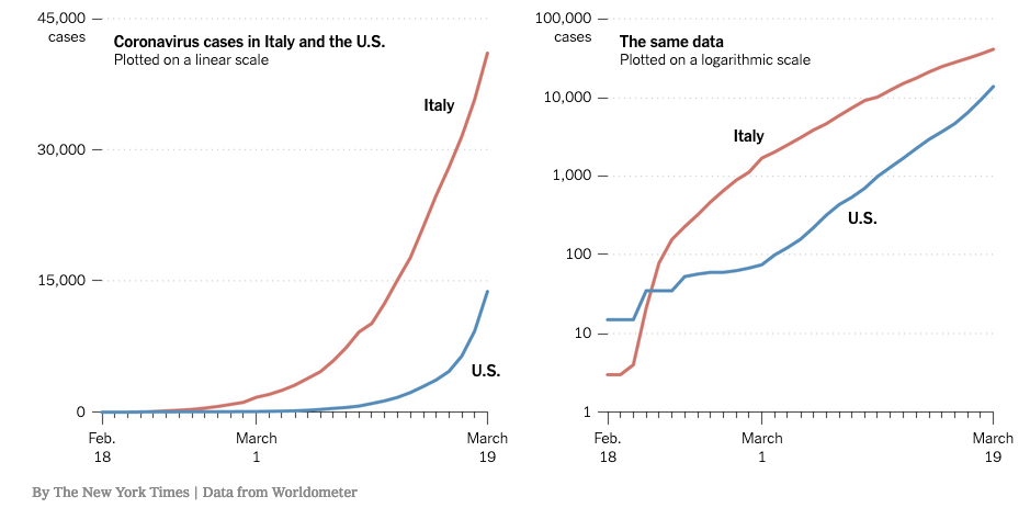
Problem 3: Recall the graph you drew for y = log x (for base 10 logs). Suppose you were to now draw the graph for . Given the relationship between the two types of logs, how would the graphs be related?

Exact relation to base 10 logarithms

To find the exact relationship between base 2 and base 10 logarithms, I just need to go back over the argument I just made, and replace all my approximate statements with exact ones.

I started out by saying that, since is about 0.3, this means that a two is worth about 0.3 of a ten:

.

I could have said that without the approximation:

.

(Say what this means in words to yourself a few times until it starts to make sense!!)

Next, I wanted to turn it around and figure out how many twos I needed to make up one ten. I said

comes up short. Well, since multiplying the numbers adds the number of tens (exponents), I’m trying to figure out

so the answer is

,

which is how I got approximately 3 and a third. But that 0.3 is just an approximation for , so the exact value is

What, exact value of what? Remember we were trying to find how many twos I need to make up one ten. The approximate answer is 3.33; the exact answer is

twos count as one ten. That is,

.

This in turn means that, if I count the tens in a number, then I have to multiply this by in order to find out how many twos there are:

.

The log base 2 of a number is just a constant value times the log base 10 of that number. The constant is approximately 3.33, and it is exactly .

Bases other than 2

If we were to start counting the number of threes in a number, the whole discussion above would go pretty much the same. We would be computing the “logarithm base 3”. We would end up with the relation

;

if we work out the numerical factor in front on the right side, we would get

.

Similarly, if b is any positive number, the log base b is related to log base 10 by

.

A handy case to remember is the conversion for natural logarithms, base e, which we’ll talk more about a bit later. The rule is

;

numerically, this works out as

,

which is quite useful for computing natural logs mentally. For example, if I want to find ln(3700), I first mentally estimate log(3700)=3.57 (right?? check my math!), and then multiply by 2.30. Here’s my method for multiplying mentally by 2.3:

First multiply by 2. I know 3.50 x 2 = 7; then, 0.07 x 2 = 0.14.
So 3.57 x 2 = (3.50 x 2) + (0.07 x 2) = 7 + 0.14 = 7.14.
Then, multiply by 3: since I’ve already multiplied 3.55 by 2, I just add one more:
3.55 x 3 = (3.55 x 2) + (3.55 x 1) = 7.14 + 3.55 = 10.69.
Now move the decimal point:
3.55 x 0.30 = 1.069, or roughly 1.07.
Finally, I add 3.55 x 2 plus 3.55 x 0.30:
3.55 x 2.30 = (3.55 x 2) + (3.55 x 0.30) = 7.14 + 1.07 = 8.21.
So, my estimate is ln(3700) is about 8.21.

I’m writing out many steps, but with a little practice this isn’t hard to do mentally (or at least with pencil and paper). Now, there is an ln key on the calculator, so I can check this! I enter ln(3700), and get:

Ha ha, that’s just my cat. Let me try again:

That’s better! My mental estimate was 8.21, so things are going pretty well.

Problem 4: Compute the natural log of each of these numbers approximately. Do it mentally by finding the log of the number base 10, and then multiplying by 2.30. Check each answer on a calculator.
a. 10
b. 1,000,000
c. 73,368
d. 0.002

Applications of logs with different bases

Why would we use bases other than 10?

Base 2 is useful in applications where it is natural to talk about doubling or halving things. In population growth, cell growth, epidemiology, and other similar growth problems, exponential growth is typical in early stages, and people like to express things in terms of “doubling time”. Therefore log base 2 is helpful. In problems of radioactive decay (like carbon dating), the decay is exponential, and people like to talk about the rate in terms of “half-life”, so, again, log base 2 is helpful. In music, doubling the frequency (multiplicatively) of a tone increases the note (additively) by an octave. So logs are involved, and in particular log base 2 is the sensible one, since doubling a frequency is the most important relationship between notes harmonically.

It will be easier to give more detail about application of and once I tell you a bit more about logs and equations, in “Logarithms Version 3” that is coming up soon. Once we have that, I’ll give you some more detail for some of them.

Logarithms base e, “natural” logs, appear in all sorts of places, particularly in physics and in probability, but many other surprising places too. The reason for using such a strange base, e=2.71828182845904523536028747135…, depends on calculus. The calculus story also gives a whole different way of motivating logarithms. To get the full story, you’ll need to take calculus here! But I will try to at least give you the beginning of the story, towards the end of these lectures.

Optional Appendix: What is special about 10?

You can skip this section if you like. It isn’t needed in anything after this.

Why DO we start with logarithms base 10? It’s particularly easy to compute logarithms in base 10: if you see the number 12,760,368, you know right away that its logarithm base 10 is between 7 and 8, and a little thought can give you a more accurate estimate. What is the logarithm of 12,760,368 base 2? That’s much harder to see immediately; you would have to know your powers of 2 up that high to see it directly. The easiest way to find the base 2 logarithm of a number like that is to find the base 10 logarithm and convert.

But why should 10 be easier? It’s because our numbering system is based on tens.

There is nothing mathematically special about 10. Ten is a historical accident: some 500 million years ago (biologists can correct my date!), there were a bunch of different body plans in competition, and the one which one and led to vertebrate life happened to have five things on the end of each appendage, rather than some other number.

Consequently, we group things every ten. And then once we have ten groups of ten, we group that too, so we count in groups of 10 x 10 = 100, and so on. The number 3,148 means 8 single things, 4 groups of 10, 1 group of 10 groups of 10, and 3 groups of 10 groups of 10 groups 0f 10:

3,148 = 3 x (10 x 10 x 10) + 1 x (10 x 10) + 4 x (10) + 8

Actually, even with our fingers, using 10 is a historical accident: at various times, people have also grouped in groups of 20, 60, and 12. In modern times, people have used groups of 2, 8, and 16, for computer reasons. If the Mayan society had been more long-lived, we might be counting in groups of 20 today.

For example, if we used 8 as the basis of our number system, we would count

1, 2, 3, 4, 5, 6, 7, 10, 11, 12, 13, 14, 15, 16, 17, 20, 21, …

In this system, “10” doesn’t mean ten; it means eight: 1 group of eight, 0 singles. The number “37” in base 8 means 31 in our system: “37” means 3 x 8 + 7 x 1. The number “2457” means

“2457” = 2 x (8 x 8 x 8 ) + 4 x (8 x 8 ) + 5 x (8) + 7

Base 8 only has 8 symbols: 0, 1, 2, 3, 4, 5, 6, 7. There is no need for a symbol for 8 or 9.

If we used a base bigger than 10, we would need more symbols. In base 16, the standard way people count is

1, 2, 3, 4, 5, 6, 7, 8, 9, A, B, C, D, E, F, 10, 11, 12, … , 1E, 1F, 20, 21, ….

The letter “A” stands for 10, “F” stands for 15. For example, the number “D4” stands for 13 groups of 16 plus 4 singles (so equals 212 in decimal notation).

Let’s try base 2 (also called “binary”). We would count (decimal on left, binary on right):

1 = “1”
2 = “10”
3 = “11”
4 = “100”
5 = “101”
6 = “110”
7 = “111”
8 = “1000”
9 = “1001”
etc.

So, for example,

.

If this seems strange, it’s just because we aren’t used to it; if we were used to counting in base 12, say, then base 10 would seem just as strange and complicated. There is nothing mathematically special about 10.

How is this related to logarithms? Well, check this out. The numbers I am writing in quotes are in binary; numbers without quotes are ordinary decimal notation:

…

The logarithm base 2 IS counting the zeroes—but it’s counting the zeroes when the number is written in base 2!

So if I write my numbers in base 2 notation, then I could do the whole development that I did from the beginning: counts the zeroes, then figure out how to interpolate, etc etc. Logs with any whole number base b can be thought of as counting the zeroes, when you are using the number b as the basis for your counting system. (But this isn’t going to work quite as nicely for logs base e!!)

In this lecture, I want to connect what we have been doing with scientific notation (which I’ll define for you if you haven’t seen it). I also want to give some examples of how logs are used to understand large numbers, make estimates, and do mental calculations.

Scientific Notation

First, let me remind you of exponent notation. The notation means multiply 10 by itself, x times:

and so forth.

This means that, in the way we were talking about before, the number has x zeroes. Well, we can then extend this. We decided that 3 has roughly half a zero, so we could write . (And if you recall our discussion about that, the number that has exactly half a zero is the square root of 10: exactly.)

When we were calculating logs, we started by rewriting the number in the form of a number between 1 and 10, times a multiple of ten. For example, in finding the log of 63,536, the first step was to write

The name for this way of writing a number is scientific notation. There are many advantages to writing a number this way. The most important part of a number for many purposes is its rough size, that is, how many zeroes it has; writing 63,536 this way, we are saying that it is “4 plus a bit” zeroes.

Finding the log takes this a step further; it encodes the entire number in the number of zeroes. We estimated that ; checking on a calculator, we find that , to four decimal places. So the number 6.3536 contributes 0.8030 zeroes; we could write

,

which means

;

the number 63,356 is 4.8030 zeroes, to four decimal places.

Scientific notation is a very standard way of writing numbers in technical work. Writing them as their number of zeroes—as their logarithm, or their power of ten— is not so standard. But thinking of them this way is quite standard, and gives some common and useful tricks for understanding and working with large or small numbers.

Problem 1: Write each number (i) in scientific notation, and (ii) approximately as a number of zeroes (that is, power of 10) (do this without a calculator).
a. 585
b. 656 billion
c. 3,500,000
Make up some more numbers to do this with, until you get the hang of it. (This is really no different from computing logarithms of the numbers. I’m phrasing it slightly differently, but it’s the exact same computation.)

Estimations and Fermi Problems

In order to talk intelligently about problems involving large numbers, it is necessary to have some intuition for what is large or small in your particular context. For example, in talking about national or international policy problems, it is common to talk about costs in millions and billions and trillions of dollars. Without a little training, these numbers all sound like “really huge or whatever”. But it is very important to understand what is truly large for a given context, and what just seems large.

Part of this is just experience; people who think about, say, education policy, have a sense of what 10 million dolllars will buy, versus 100 million or a billion. These numbers just seem “big”, but 100 million is ten times 10 million. If you hear a building cost 10 million or 100 million to build, it sounds sort of the same. But if you go to buy a can of soup, and you have a choice between one that costs 2 dollars and one that costs 20 dollars, you know the difference!

Aside from having actual experience buying multi-million dollar things, another way to build intuition is to get in the habit of estimating. Thinking in terms of logarithms and number of zeroes helps with this.

Here’s an example: let’s guess the GDP of the United States. GDP is “gross domestic product”: roughly speaking, it is the value of all the goods and services produced by every person and company in the US per year. It’s not easy to guess off the top of your head, but it’s easy to get an estimate.

Start with the population of the US, a number everyone should know: about 300 million. (Not exactly, but I’m estimating here.) That is 8.5 zeroes (). (Right!? Check my math!)

Now, how much does everyone make? What’s the average salary? I’m going to say 30,000 a year. Now, I might be off: maybe it’s 50,000. But I’m just trying to get the number of zeroes right. How many people are actually working? I’m going to guess 200 million. Again, I could be off, but I’m aiming to get the right number of zeroes.

So, we have 8.3 zeroes () number of working people, each making 4.5 zeroes () dollars each per year. For total dollars made per year, you multiply; but multiplying adds zeroes. So the total income is 8.3 + 4.5 = 12.8 zeroes worth of dollars per year, dollars per year.

Now, that was income. But GDP was supposed to be output. Now, people aren’t going to make in income what they produce in output: the corporate parasites capital investors are going to be making profits. That means the GDP will be bigger than income by some factor, which takes into account all the extra money businesses and corporations are making. I’m going to make a rough guess and say this factor is 3; that incomes are about 33% of GDP. So I should multiply my final number by 3, that is, I should multiply by , that is, I should add 0.5 zeroes.

(I don’t really know this; I’m just guessing. But here’s how I’m guessing. I don’t think total incomes are 100 per cent of GDP: businesses and corporations are making a lot of money. But I do think that personal incomes are a substantial chunk of GDP; I don’t think they are as small as 10 per cent of GDP. So I am picking half way between 10 per cent and 100 per cent; but half way in the multiplicative sense, so I’m guessing about 30 per cent, or one third.)

So in the end, my guess for GDP is 12.8 plus 0.5 zeroes, or 13.3 zeroes; that is to say, dollars. Now, 12 zeroes is a trillion, and 1.3 zeroes is about 20 (why?), so I get an estimate of

US GDP is about 20 trillion dollars per year.

Wikipedia says:

Ha!

(I didn’t look this up beforehand, honest.)

The counting of zeroes may seem a little foreign at first, but it is a very common practice among scientists who need to regularly work with large numbers. For one thing, it makes huge numbers manageable: for example, the number of atoms in the entire observable universe is something like or , so our brains never have to manage numbers bigger than 80 (and usually smaller ones). For another thing, in problems like this, we are almost always multiplying, which is difficult both for doing mentally and for having an intuition. But number of zeroes (the logarithms of the numbers) add rather than multiply. Adding is easier.

So, this whole process seems a little weird and difficult at first, but it becomes very quick and easy with practice, and is valuable in all kinds of places. Getting in the habit of doing this will give you a facility with and intuition for very large and very small numbers, which can be powerful.

Problem 2: Make an estimate of the total US consumption of oil per year. (Hint: You could start with cars. Guess how many miles each car owner drives, and miles per gallon. Then guess what percentage of oil consumption goes to cars. There are other ways to approach it too, but try to work from things you can reasonably guess. Don’t be too fussy; being off by a factor of 2 or 3 in places is to be expected. We’re just trying to get the number of zeroes right.

Once you have an answer, look up the actual figure, and see how close you got.

This method can also be useful for mentally calculating large numbers, where you could in principle find an exact answer, but all you want is a rough answer.

For an example: most Vermont license plates consist of three letters and three numbers.

How many license plates are possible in principle? Well, there are roughly 26 choices of the first letter (probably they avoid using letter “O” or “I”, and some vulgar combinations, but I won’t worry about that). For each choice of first letter, there are 26 choices of second letter, so 26 x 26 choices for first two letters. Continuing this way, the number of license plates is

26 x 26 x 26 x 10 x 10 x 10.

Don’t reach for the calculator yet! I want to show you how a scientist does this immediately mentally.

The numbers are easy: each digit gives one decimal digit of information, that is one zero. So the 10 x 10 x 10 gives 1,000 , that’s easy.

How many decimal digits of information are contained in a letter? That is, how many zeroes is 26? Using our methods, you should see that log(26) is about 1.4 or so. So each letter contributes 1.4 zeroes. (More formally, .)

The letters give 1.4 + 1.4 + 1.4 = 4.2 zeroes, and the numbers give 3 zeroes, so we get 7.2 zeroes total. Then, 7.2 zeroes is roughly

17 million different license plates possible.

(Right? How did I convert 7.2 zeroes back into a number?)

Let’s check by putting 26 x 26 x 26 x 10 x 10 x 10 in a calculator:

Problem 3:
a. Calculate the approximate number of seconds in one year, using this logarithm method. Don’t use a calculator. Once you get your answer, though, check it on a calculator.
b. How many seconds old is the universe? (The universe is about 13.8 billion years old, according to current theories and measurements.)

So far, we’ve figured out how to mentally estimate the log of any number greater than 1. What about numbers less than 1? I want to explain how that works, including what happens with 0 or with negative numbers.

First let’s review so far: the logarithm “counts the zeroes” in a number. For a multiple of ten, that is literally true:

log(10) = 1
log(100) = 2
log(1,000) = 3
log(10,000) = 4
log(100,000) = 5
log(1,000,000) = 6
etc.

For numbers that aren’t multiples of ten, we have extended the idea of “number of zeroes”, by using the fact that multiplying numbers will add the number of zeroes: for any two numbers a and b,

log(a x b) = log a + log b.

In words: the “number of zeroes” in a x b is the “number of zeroes” in a plus the “number of zeroes” in b.

For example, the number 3.16 roughly represents half a zero, because

3.16 x 3.16 = 10

approximately. (We are often just rounding this to 3.) Written using the fundamental rule above:

log(3.16 x 3.16) = log (10)
log(3.16 x 3.16) = 1
log(3.16) + log(3.16) = 1 (using the fundamental rule)
so log(3.16) = 1/2 (approximately).

I asked you to find log(1) in a problem above. In case you ran into trouble, here’s how the solution goes:

1 x 10 = 10
so log(1 x 10) = log (10)
so log(1) + log(10) = log(10)
so log(1) + 1 = 1
so log(1) = 0 (after subtracting 1 from both sides).

Therefore log 1 = 0. The number 1 counts as having “no zeroes”. Multiplying 1 by a number doesn’t change it, so it doesn’t add anything to the number of zeroes.

(Note that I could have used any positive number in place of 10 in the argument above; the only reason I used 10 is because I know log(10), but in fact I didn’t really need it: I could have subtracted a log(10) from both sides one line earlier than I did.)

The logs of positive numbers which are less than 1

OK, so what about a number less than 1? Since we’re going with multiples of 10, let’s try 0.1 first. I need to relate 0.1 to something I already know the log of. And I should use multiplication, because I want to use the fundamental rule. So, I’m going to start with

0.1 x 100 = 10.

(That isn’t the only thing I could have started with. In what follows, try something else in place of 100, and see if it works out!)

So now, following the same sort of strategy I’ve been doing so far:

log(0.1 x 100) = log(10)
log(0.1) + 2 = 1
so log(0.1) = -1.

(I skipped steps this time; can you fill them in?)

So, 0.1 counts as “1 negative zero”. Or an “antizero”. You can see that more informally from

0.1 x 100 = 10;

multiplying adds the zeroes. So I added some number of zeroes to 2 zeroes, and got 1 zero as a result. I must have added -1 zeroes.

Problem 1: Find the following. (Even if you have a reasonable guess for what these are, please write out the reasoning. You can either reason like I did for log(0.1); or you can use log(0.1)=-1, and use the fundamental rule.)
a. log(0.01)
b. log(0.001)
c. log(0.0001)
d. log(0.00001)

Problem 2: Find approximate values for the following, without a calculator. Once you find them, check your answers with a calculator.
a. log(0.7)
b. log(0.5)
c. log(0.0035)
d. log(0.00008)

Hopefully you can see that you can now mentally approximately calculate the log of any positive number, no matter how big or how small.

The log of zero??

What you have figured out above should tell you that something weird is going on with the log of zero.

Problem 3:
a. The logs you found in Problem 1 of this lecture are logs of numbers that are getting closer and closer to zero (0.1, 0.01, 0.001, 0.0001, etc.). What does this suggest about the value of log(0)? Why should that make you worried?
b. Remember the graph you did of y=log x? The one where your x range went from 0 to 10, but you could only fill it in starting at 1? Take the values you found in Problem 1, plot the corresponding points on the graph of y = log x, and use them to extend your graph. What is that suggesting about log(0)?

Problem 4: Undeterred, we might try to figure out log(0) directly. We could use a similar strategy to what we tried above: we could start with an equation like, say, 0 x 10 = 0, and follow similar steps to try to find log(0). What happens when you carry through this strategy? You should get a troubling result: what do you think this troubling result means??

The log of negative numbers

If you remember logs from high school, you might recall that it was always forbidden to take the log of a negative number. There are good reasons for this in the high school approach. However, whether logs of negatives makes sense depends a bit on your definitions, and on what you want to use logs for. I’ll come back to this point later. But for the moment, I want to note that, according to our reasoning in this first version of logs, the logs of negative numbers are actually totally fine.

Problem 5: Use the fact that (-1) x (-1) = 1, and the fundamental rule for logs, to find the value of log (-1).

Problem 6: Use the value you found for log (-1), plus the fundamental rule, to find:
a. log (-10)
b. log (-100)
c. log (-1,000)

Problem 7: Based on what you were just doing, you hopefully saw a simple rule. If x is any positive number, state the rule for what log(-x) is. (You should be able to state it as a formula.) Explain why your rule is always correct (your explanation should take the form of some equations).

There are three parts to this Lecture (which mostly consists of problems for you to work through). The first is to understand what the graph of the logarithm function looks like. The second is to see how using a log scale affects a graph of another function mathematically. The third part is to see how this can work with practical data.

The graph of the logarithm function

For these problems on graphing, ideally you will have some graph paper available. If you don’t, and you have a printer, there are a number of sites that offer free pdfs of graph paper that you can print out. If you have neither, you can use blank or lined paper and a ruler.

The graphs should be somewhat careful and accurate, but don’t have to be super-accurate.

I would prefer that you do not use a computer to make these graphs. Creating the tables and the graphs by hand helps give you an intuition for them, that you don’t get the same way on the computer. However, if you are really stuck for supplies, or have issues that make graphing on paper impossible, a computer graphing program could be used as a last resort.

Problem 1: You have already created a table of values for y=log x, where the x ranges through 1, 2, 3, …, 10. Use these values to make a graph of y=log x, wher x ranges from 0 to 10. Try to plot fairly carefully. Choose a range for your y-axis which makes the graph a reasonable size, then split up that range into equal parts (in an additive scale!). Plot the points, then connect them with a continuous curve. (We haven’t addressed what happens with log 0, so your graph will actually start at x=1. If you don’t know already, you might make guesses about what happens to the left of x=1.)

Problem 2: Make a graph of y=log x, for an x range of 0 to 100. Figure out how much y range you need, and then pick your y scale accordingly. Be sure to use an ordinary linear scale for the x and y axes. Make a table of values, for a reasonable number of x values. I would suggest computing the values of log x mentally, to give you practice, but you can check them on a calculator.

Problem 3: Make a graph of y=log x, for an x range of 0 to 10,000. What is this telling you about the logarithm function?

Using a log scale to transform other graphs

A common application of logarithms is to transform data. I would like you to see how it works with exact mathematical functions first; then we’ll try it on empirical data.

Problem 4: Make a graph of the function . Make your x range from 0 to 10. Figure out how big a y range you need, before you start graphing! Make your table of values first. Make your y range so the biggest value will fit on your page, then split up your y scale accordingly. Be sure to use an ordinary linear scale for your y axis (going up by constant additive steps).

Problem 5: Now, I want to make another graph of , but this time I want to use a logarithmic scale for the y axis. The top of your scale will be 1000. Then, you should mark 1, 10, 100, and 1000, with even spacing between each. I’d like you to mark the halfway point between each of these markings as well; according to what we did before, what numbers should those be labelled with? Now, use your same table of values for , and plot the points.

Problem 6: I want to make one more graph of . This time, though, I want to graph, not y, but log y. On your table of values, for each value of y, find log y. See what the biggest value of log y is, and pick a range for your vertical axis accordingly. Split up your vertical axis in a linear scale (so if 3 is your top, then 0, 1, 2, and 3 should be evenly spaced on your vertical axis). Now plot the points: plot x versus log y, where . Compare this to the previous problem; what is the difference?

Using a log scale to transform real-world data

In class, I introduced you to the gapminder.org site. They have an amazing array of real-world data, and data visualization tools that you can use.

Here is life expectancy as a function of income (measured as GDP per person, adjusted for purchasing power; click on “Data Doubts” at the bottom right of the graph on their site for more details):

Note that the data is all crowded towards the left side of the graph. More significantly, the x axis is not really evenly spaced in practical terms. It is evenly spaced mathematically, additively: each marking is the equivalent purchasing power of 20,000 US dollars. So the spacing is 0, 20,000, 40,000, 60,000, 80,000,… But this isn’t evenly spaced in terms of life realities. There is a vast difference between living on 1,000 a year and 21,000 a year; that difference is far greater than the difference of living on 80,000 a year versus 100,000 a year. The additive difference is the same in both cases; but what is practically more relevant is the percentage changes, or multiplicative difference.

When you in a situation where percentage or multiplicative differences are the important thing, it is usually a good idea to use a log scale for that variable–or, equivalently, to graph the log of that variable. What is practically important is not the income, but the log of the income.

The reason is that we really only understand additive changes well; if something behaves by multiplicative changes, then it is usually a good idea to use the logarithm to convert multiplicative changes to additive changes, which we can see better.

We can do this on the gapminder graph by selecting the little arrow next to the “Income” label on the x-axis, and selecting a “log” rather than “linear” scale:

Now, there is a linear trend apparent in the data. This means that any fixed percentage increase in income will, on average, create the same additive change in life expectancy. People often express this as doubling: each doubling of income adds xxxx years to life expectancy, on average.

Now, you might wonder why I didn’t use a log scale for life expectancy. Practically speaking, it seems that life expectancy is really a linear thing: each additional year is an additional year. It’s not so dependent on percentage changes as income is. However, this is a somewhat subjective judgment call in many cases, and it can depend on what you’re trying to see in the data.

Problem 7: In the second graph shown above, find the log of each marking on the x axis. In this way, verify that the x axis is additively evenly spaced if we are showing log x (i.e. log income), rather than x itself.

Problem 8: If you click on the axis labels on the graph in gapminder, you find that there are wide variety of different variables that they have data for, and which you can graph. Select two variables to graph (other than life expectancy versus income), on the following criteria:
– one variable should seem to you that it is multiplicative in its practical nature: that percentage changes in that variable matter more than absolute changes
– the other variable should seem to you that it is additive in its practical nature
– the two variables and their relationship should seem interesting to you
Pick one of the variables to be x, and the other y. (Usually the convention is to make y the variable that you think of as “dependent”: you are thinking of the y as depending on the x. In the real world, of course, the causal direction may not be that simple, but make a judgment there.) Make two graphs: make one with a linear scale for both variables; make another with a log scale for the variable you think is multiplicative, while keeping a linear scale for the variable you think is additive.

Take a screenshot of each graph so you can refer back to them. Explain what you think is differently visible in each graph.

Problem 9: The same thing as Problem 8, but this time, pick two variables for which you expect both of them to be multiplicative. This time, make three graphs: one with linear scales for both variables; one with a linear scale for one variable, log for the other; and finally, one with log scales for both. As before, take screenshots, and compare the results.

OK, so now I want to go back to figuring out some more logarithms, at least approximately. By the end of all of this, you should be able to figure out the logarithm of any number, in your head, correct to at least one decimal place. This will also give you some practice with the fundamental rule for logs (see the colored box below).

Logs of numbers 1, 2, 3, … , 10

Recall from the last lecture that we decided that the number 3 represents approximately “half a zero”, since , and multiplying numbers adds the number of zeroes. The logarithm counts the zeroes, so . (Actually a little less than , because if 3 was exactly half a zero, then 3 x 3 would be exactly 10.)

We can state this a little more mathematically. I’ve said that multiplying numbers adds their number of zeroes. And “log” counts the number of zeroes. So, for example,

log(100 x 1,000) = log(100) + log(1,000)

says, in words, that the number of zeroes in 100 x 1,000, is the number of zeroes in 100 plus the number of zeroes in 1,000 (so 5 = 2 + 3).

In fact, for any two numbers a and b, the number of zeroes in a x b should be the number of zeroes in a plus the number of zeroes in b:

This is super-important. This is a mathematical way of saying what I’ve said in words, that logs convert multiplication to addition. I’m going to keep coming back to this rule over and over.

This rule allows me to make my argument above look more mathematical. I am setting a=3 and b=3 in the rule. That is, since

,

we have

,

so

,

but by the fundamental rule:

,

which means that

.

Let’s try to find log 2 in a similar way. We know that

,

where that “approximately equals” is pretty rough this time. That means

,

and by our fundamental rule, log(2 x 2 x 2) = log 2 + log 2 + log 2. So we know

,

so log 2 must be roughly . It is not exactly , because if it was, then 2 would be “ of a zero”, and 2 x 2 x 2 would be exactly 10. So log 2 must be a bit less than . We could guess

,

say.

In fact, we can justify this another way. A little experimentation will show that

2 x 2 x 2 x 2 x 2 x 2 x 2 x 2 x 2 x 2 = 1024,

which is pretty close to 1000. (That’s ten twos multiplied.) Using the rule as we did before (fill in the details!), we end up with

,

so

.

This gives us the estimate

.

(Please fill in the details yourself to make sure you understand!)

So, as we go forward, remember the estimates

and remember always the fundamental rule,

Problem 1: Find an estimate for log 4. (Hint: you already have an estimate for log 2; use the fundamental rule.)

Problem 2:
a. Find an estimate for log 6. (Similar hint.)
b. Find an estimate for log 8.

Problem 3: You can find an estimate for log 5 in two ways. (Please do both! They are both informative in different ways.)
a. Make a guess based on your estimates for log 4 and log 6.
b. Use the fact that 2 x 5 = 10, and use the fundamental rule.

Problem 4: Find an estimate for log 7. (Try to do it two different ways, similar to the previous question.)

Problem 5: Now find an estimate for log 9. This one is easiest to do like Problem 3a; I don’t know an easy method like Problem 3b for this one (you can look for one if you would like a challenge problem!).

Problem 6: You know log 10 already. (Right?! Check back if you don’t recall.) The only whole number from 1, 2, 3, … , 10 that we are missing is log 1. It’s a little tricky, so I’ll give away the answer: log 1 turns out to be zero. Use the fundamental rule to show that log 1 has got to be zero.

Problem 7: Finally, summarize all your results. Make a table:

Number:	1	2	3	4	5	6	7	8	9	10
Log:		0.3	0.5

Fill in the rest of the blanks!

Estimating log of any number (larger than 1)

We can use what we’ve done to approximately find the log of any number. (For now I’ll concentrate on numbers larger than 1; I’ll get to smaller numbers later.)

For an example, let me pick a number at random: say, 63,538. What is the log of this number? I know that the number is between 10,000 and 100,000, so it “has 4 point something zeroes”. That is, log(63,538) must be between 4 and 5.

To find out more closely where it lies between 4 and 5, rewrite the number 63,538 as

6.3538 x 10,000

which I’ll round off to

6.4 x 10,000.

That factor of 6.4 is telling us how far we are between 4 zeroes and 5 zeroes, in a multiplicative sense:

So, the log(6.4) is giving us the decimal part of “4 point something”. Now, we have established that , and , so I’m going to guess that . This finally leads to the estimate

.

Let’s check it:

Not bad, right? (See Problem 10 below on how to make the estimate a bit better.)

So, to calculate logs mentally, one way to go is to memorize the logs of 1, 2, 3, … , 10, and then use the method above. My own way is to just memorize and , and to figure out the rest of 4, 5, …, 9 as I need them, doing it like you did in the previous problems.

Problem 8: Find the log of each of the following numbers approximately, doing the calculations mentally.
a. 560
b. 4160
c. 31,000,000
d. 72,380,000,000
e. 13,468
Check your answers with a calculator! (On some calculators, the “log” we are using is written “.”)

Problem 9: Make up some more numbers at random, and calculate the logs of them. This is a good exercise to do while doing something else. You can also do this with a partner: one person makes up a number, the other person works out the log. Note that the numbers can be enormous if you like–that doesn’t make it harder to find the logs. Practice this until you can do it fairly easily.

Problem 10 (optional): You saw in the example above, where I tried to calculate log(63,538), that I was a bit off. The main reason for this is log 3. Our estimate of log 2 was 0.3; the actual value (to four decimal places) is log 2 = 0.3010, so 0.3 is pretty good. But we estimated log 3 = 0.5, and that is a bit off; the actual value is log 3 = 0.4771.

If you want to be accurate to about two decimal places, you can remember , as above, but remember , and figure out the other values from these.

Use those two values to recalculate logs of 4, 5, 6, 7, 8, and 9, and make a more accurate version of the table from Problem 7. Use those numbers to re-do the example of log(63,538) that I did above, and see how much closer you get.

(If you want to do even better, you can memorize and …)

In this class, I am going to introduce logarithms multiple times, in multiple different ways. Most of these ways of seeing logarithms have a central property in common:

Logarithms transform multiplication into addition.

I’ll have a lot more to say about this as the course progresses. Keep this in the back of your mind as we start on this first version.

Counting zeroes

This first version is the easiest. The logarithm just counts zeroes. So, the log of the number 1000 is 3, because the number 1000 has 3 zeroes.

We write this:

• 
• 
• 
• 
• 
• 
• 
• and so on!

And that’s it!

Well, no, not entirely it. There are probably two questions that occur to you at this point. For one thing, what if the number isn’t a nice round number like 1,000,000, but something more like 31,648? And secondly, what is the value of doing such a simple-minded thing in the first place?

I’ll try to start answering the first question now. The second question will be answered gradually throughout the class, but I’ll give a teaser at the end of the post.

How to interpolate log

So, what should the log of a number like 32 be?

There are many different answers you could give to this question. You could say log(32) just isn’t defined: log(10)=1, and log(100)=2, but the number 32 has no zeroes. You could alternately say that the log of every number from 10 up through 99 is equal to 1, and then it jumps to 2 when you get to log(100). So by that reasoning, log(32) would equal 1.

So, there isn’t just one answer to what log(32) should be. But I’m going to try to find an answer that makes the most “sense” (where “sense” is a bit subjective!). This is a question of “interpolation”: how do I fill in the missing values of log continuously?

Since log(10)=1 and log(100)=2, and since the logs are getting bigger as the number gets bigger, I’d like to say that log(32) should be a decimal number between 1 and 2.

Moreover, I’d like to say that for all numbers x between 10 and 100, the value of log(x) is between 1 and 2, and that it gets bigger as x gets bigger. So, log (15) should be pretty close to 1, and log(95) should be pretty close to 2. But how do I fill in the numbers exactly?

I could fill them in proportionally. For example, since 55 is halfway between 10 and 100, I could say log(55) should be halfway between 1 and 2. That would mean l0g(55)=1.5. I could figure out other logs similarly. But this procedure ends up not making as much “sense” as I would like. In particular, if I make this definition, I end up getting a graph for log(x) that has straight line segments connected by sharp corners – a sign that something is weird.

Let me try asking a different question: what is a half a zero?

Multiplying numbers adds the zeroes

What would be a number with one and a half zeroes? Would it look something like this?

Well, look at what happens when we multiply multiples of 10. For example, if we multiply 100 x 10,000 we get 1,000,000: two zeroes plus four zeroes equals 6 zeroes. Multiplying the numbers adds the number of zeroes.

So if we multiply a number with one and half zeroes by itself, the two half-zeroes should combine to make a whole zero, and we should get three zeroes in total:

That is, multiplying a number with 1.5 zeroes times a number with 1.5 zeroes should give 3 zeroes total.

Now, what is such a number? It is a number that multiplies by itself to give you 1000? What could that number be? Well, we can start guessing and checking:

• 30 x 30 = 900
• 31 x 31 = 961
• 32 x 32 = 1024
• 31.5 x 31.5 = 992.25

So, a number with one and a half zeroes is a little bigger than 31.5.

Problem 1: find this number more accurately!

(If you recall your math, this number has a name: it’s the square root of 1000. But it’s instructive to find it by guess and check nevertheless.)

So now we’ve figured out something about logs! Since log(10)=1, and log(100)=2, and since one and a half zeroes is about 31.5, we have concluded that

Working even more approximately (which I want to do for now), we could say that

Another way of saying this: halfway between 10 and 100 is 55 in the additive sense, because

10+45=55, and 55+45=100.

But halfway between 10 and 100 is about 31.5 in the multiplicative sense, because

10 x 3.15= 31.5, and 31.5 x 3.15 = 100.

More roughly speaking, halfway between 10 and 100 is about 30, in the multiplicative sense.

What is this good for?

Before I develop this further, what is the point of this? I’ll try to give a number of different answers in this class. Here’s one which is unfortunately very relevant right now:

In the initial stages of a spreading infection, we expect the number of cases to grow multiplicatively: one person infects two, those two each infect two, those four each infect two… So we expect the number of cases to be multiplied by a certain fixed factor each day. Or said differently, we expect the number of cases to double in a fixed number of days. This is what the phrase exponential growth means.

It is difficult to read rate of growth clearly on a graph when it is exponential: it shoots up too fast. But there is another way of graphing. On the y-axis, we have always been taught to space the labels evenly. That is what happens on the graph at left: each spacing is 15,000 additional cases.

But that is spacing evenly additively. What if we space evenly multiplicatively? Then each marking on the y axis should be a constant multiple of the last one. That’s what is shown on the graph at right: each equally spaced marking on the y axis is 10 times the previous one.

In other words, the y-axis is evenly spaced, counting the number of zeroes: the lines are 1 zero, 2 zeroes, 3 zeroes, etc. In yet other words, the y-axis is showing the logarithm of the number of cases.

On such a graph, an exponential growth is going to be a straight line. (We will see exactly why this is true soon, but hopefully that seems at least plausible to you now.) So we can more easily see deviations from exponential growth. We can see that, as of mid-March, Italy was beginning to succeed at “bending the curve”, whereas the US was not successful at this yet. This is not evident from the graph at left.

I encourage you to read the article I took this graph from. (I believe this article should be free to access, but let me know if not, and I’ll send you a copy.) You can see more detail for different countries at this Financial Times article by Steven Bernard, Cale Tilford, John Burn-Murdoch and Keith Fray.

To connect this to what we started above: if we added more markings to the graph on the right, we would make the multiplicatively evenly spaced. So if we wanted to add an additional marking halfway between 10 and 100, it should be marked about 31.5.

Some questions

Problem 2: What number has a half a zero? In other words, what number x has log(x) = 0.5?
(You can just give an approximate answer.)

Problem 3: Roughly, what is the value of log(3)?

Problem 4: Roughly, what is the value of log(30,000)?
(Hint: Use the fact that 30,000 = 3 x 10,000.)

Please ask questions or discuss, either in the comments here, or on our Slack channel!

Hi everyone!

My plan is to write up my planned lectures here. I may also link videos, if I have time to make them!

Please ask questions, or have general discussions with each other, in the comments sections. We can also do that on our Slack workspace. Let’s see what ends up working best.

Email me if you have questions!