Hi again!

No real reason for the picture. Just, it’s getting lonely typing and talking into a relative void! Distance learning is difficult. I miss seeing you all.
OK, let’s get started with the math.
I am going to approach this section differently than the last ones. I am NOT going to follow the book closely; the main resource will be this lecture.
This is for a few reasons. One, the author of our text is trying to do things a bit more rigorously than I want to do them at this point. I will make rough statements about approximations here, and you can find the more precise statements in the text. Second, the normal distribution is an example of probabilities on a continuous sample space, and the author is going to explain things more completely in the second volume of this book; for the moment, he is only proving what we can with the tools so far. Third, and this is more minor, I find his notation in this chapter a bit confusing. It’s adapted to his purposes later, but for our purposes it’s a little bit confusing and non-standard.
I would recommend reading and working through this written lecture, and then after you have done that, taking a browse through Chapters VII and X in the text. I will only use this written lecture for this class; you won’t need to read the chapters. However, I think it will be helpful to have a sense of what is covered in the chapters. It will help you have confidence with the book, and if you are using probability in future, you will probably at some point need the additional detail he goes into in the text.
To help you navigate, here is a list of topics I am planning to cover in this lecture:
table of contents
- Shape of the binomial distribution, and the normal approximation
- Probabilities for ranges in the binomial distribution
- Probabilities for ranges in a continuous distribution
- Z-scores
- Estimating probabilities for ranges in the binomial distribution, using the normal approximation
- The normal distribution for its own sake
- Relative standard deviation of the binomial distribution
- The central limit theorem
1. The shape of the binomial distribution, and the normal approximation
review of the binomial distribution
Recall the binomial distribution? It’s new, and you’re still getting used to it, so let me quickly remind you. We have some experiment (flipping a coin, rolling a die, finding a defective bolt, detecting a particle, etc). The experiment has some outcome we call “success”, which happens with probability p, and anything else we call a “failure”, with probability q = 1 – p . (Note that “success” isn’t a judgment; for example, finding a defective bolt might be “success”.) We assume that each “trial” of the experiment is independent from all previous trials (so this will only apply to real situations if that is at least approximately true). Such an experiment is called a “Bernoulli trial”. We repeat the experiment n times, and our question is:
Question: What is the probability of getting k “successes” in n trials?
Answer: The probability is given by $$b(k;n,p)=\binom{n}{k}p^k q^{1-k}.$$
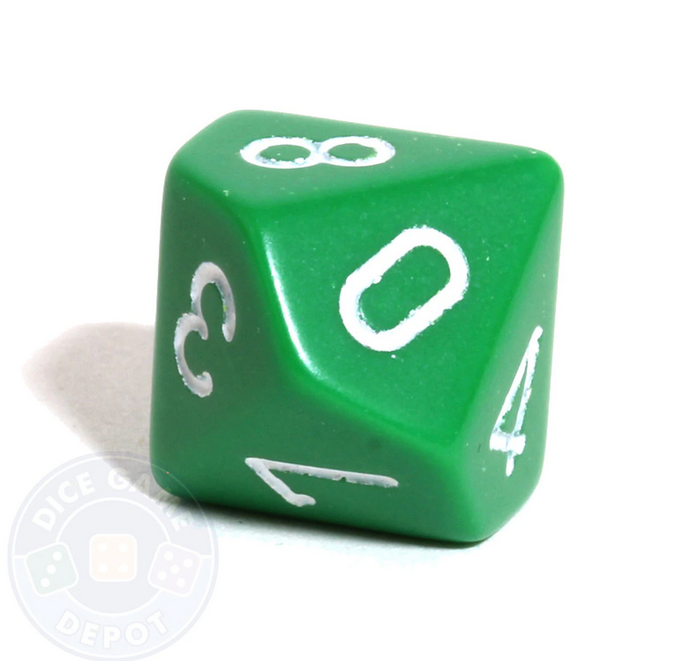
For example, let’s say we are repeating an experiment with p=0.2 of success. (Maybe we are rolling a 10-sided die, and “rolling an 8 or a 9” is a success.)
Let’s say that we roll the die 10 times. Actually, let’s assume we have 10 dice, and roll all 10 dice simultaneously (it’s the same thing). What is the probability getting no successes? It is a probability q=0.8 of failure, repeated 10 times for 10 independent dice, so overall the probability of no successes and 10 failures is $(0.8)^{10}$. That is, $$b(0;10,0.2)=\binom{10}{0}p^0q^{10}=q^{10}=(0.8)^{10}\doteq 0.1074.$$ What is the probability of one success? There are $\binom{10}{1}=10$ different ways you could get a sequence of one success and nine failures (i.e. 10 different dice that the one success could appear on), and for each of those different ways, there has to be 1 success and 9 failures, so a probability of $(0.2)^1(0.8)^9$ each. So overall, the probability of exactly 1 success and 9 failures is $$b(1;10,0.2)=\binom{10}{1}p^1q^9=10 p^1 q^9=10(0.2)^1(0.8)^9\doteq 0.2684.$$ What is the probability of two successes? There are $\binom{10}{2}=45$ different ways you could get a sequence of two success and eight failures (i.e. 45 different possible choices of two dice to be successes), and for each of those different ways, there has to be 2 success and 8 failures, so the total probability of exactly 2 successes and 8 failures is $$b(2;10,0.2)=\binom{10}{2}p^2q^8=45 p^2q^8=45(0.2)^2(0.8)^8\doteq 0.3020.$$ And so on.
If we graph all of these, you get:
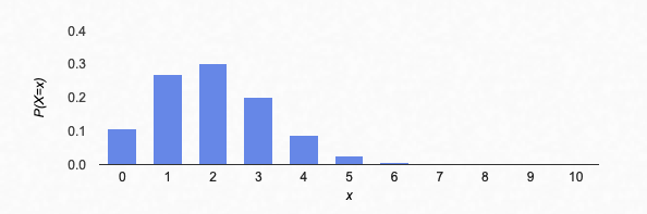
Shape of the binomial distribution
If we try larger values of n, we see that the graph of the binomial distribution looks like a continuous curve. For example, let’s try n=100, p=0.2:
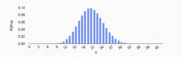
Something interesting happens: if the n is large enough, the shape seems to be the same for different values of p. It’s just centered differently, and spread out more or less.
Something I don’t like about that applet is that it automatically rescales the x and y axis, so you can’t see so well how the shape is changing. Let’s switch to something a little more powerful:
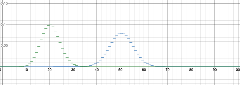
For n=100, this image compares the binomial distribution with p=0.2 to p=0.5. Note that p=0.2 is shifted to have a center at k=20 successes, which is the most likely number of successes. It is also taller and skinnier, but otherwise a similar shape.
I made the graph using Desmos, which I can strongly recommend for graphing. (Thanks Five for the idea to do this!) You can go to the graph I made above by clicking on the image, and you can drag the slider (for z, which represents p) between 0 and 1 to see how the shape changes. Or you can hit “play” to animate the change of p. I have kept the graph for p=0.5 fixed as well, for comparison. Please do this now, it’s instructive!
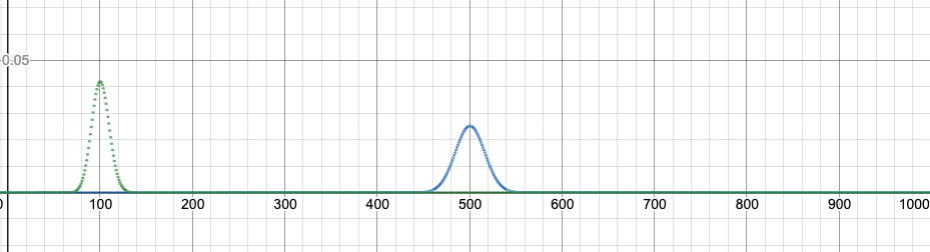
Here’s a similar graph with n=1000. I’m comparing p=0.1 to p=0.5. Click on the graph to try the slider and animation!!
What is that shape? Can we find an equation?
YES!!
I mean, yes.
The shape is the normal distribution. This is also called the Gaussian normal distribution, or just the Gaussian.
It is sometimes also called a “bell curve”, but that is misleading. There is an infinity of different functions you can make up with bell-shaped graphs. The normal distribution is a very particular function, that comes up in mathematics and nature incredibly often. Gauss first studied it in analyzing the random errors in experimental measurements (it had been studied by other mathematicians before, but Gauss was the first to identify its ubiquity). It describes quantum probability distributions, the propagation of heat, and random distributions of all sorts in nature. We’ll see one reason later in this lecture why it comes up so often—the central limit theorem—but there are many other reasons as well.
The particular shape of the normal distribution is given by the following function:
$$N(x;\mu,\sigma)=\frac{1}{\sigma\sqrt{2\pi}}e^{-\frac{1}{2}\left(\frac{x-\mu}{\sigma}\right)^2}.$$
The variable here is x (it corresponds to the k in the binomial distribution). You can think of $\mu$ and $\sigma$ as parameters, which adjust the shape of the graph.
The parameter $\mu$ (Greek letter “mu”) stands for “mean”: it determines the peak of the graph, and also the average value (we’ll define that more carefully later). (Notice that in the formula, it creates a horizontal shift.)
The parameter $\sigma$ (Greek letter “sigma”) stands for “standard deviation”. I won’t explain that now—we’ll get to it in a future chapter—but for the moment, it is sufficient to note that $\sigma$ adjusts both the “spread” and the height of the graph. Larger $\sigma$ gives a wider, flatter graph. We’ll define the concept of “spread” more carefully in the next chapter.
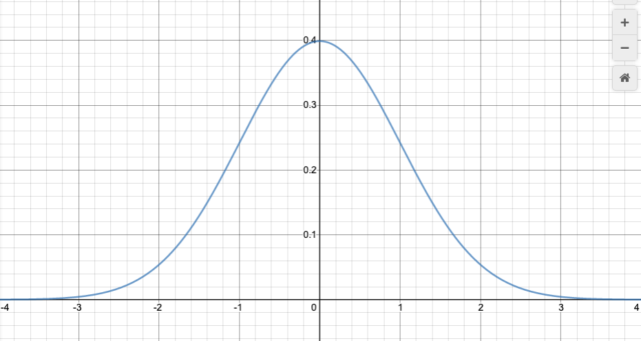
Let’s analyze it a bit for a particular case. The standard default is to take $\mu=0$ and $\sigma=1$ (we’ll see later that we can always transform to this case). Then the formula is
$$N(x;0,1)=\frac{1}{\sqrt{2\pi}}e^{-\frac{1}{2}x^2}.$$
When x=0, we get $\frac{1}{\sqrt{2\pi}}$. When x gets larger, $x^2$ gets larger, so the exponent gets more negative. The negative exponent means “one over”: $$e^{-\frac{1}{2}x^2}=\frac{1}{e^{\frac{1}{2}x^2}}.$$ That means, as x gets bigger, the exponential in the denominator rapidly gets larger, so that the overall fraction gets smaller. Increasing from x=0, the function decreases, slowly at first, and then very rapidly towards zero. The values for negative x are symmetric with those for positive x, because x appears in the equation only as $x^2$. The graph decreases the same way as we go left from x=0. Hence the “bell” shape.
Here’s what it looks like, for $\mu=0$ and $\sigma=1$:
Here’s an animation showing the effect of changing $\sigma$. Click on the image for a Desmos worksheet with a slider for $\mu$ and $\sigma$ (labeled as n and u respectively on the sliders) that you can manually change to see how it affects the curve.
The normal approximation to the binomial distribution
Now, here are the magic formulas:
$$\mu=np$$
$$\sigma=\sqrt{npq}$$
What do I mean by that?? I mean that I can fit the normal distribution function $$N(x;\mu,\sigma)$$ to the shape of the binomial distribution $$b(k;n,p)$$—very accurately, in fact, if n is large—by choosing the parameters in $N(x;\mu,\sigma)$ to be $\mu=np$ and $\sigma=\sqrt{npq}$ (remember that $q=1-p$).
Let’s try an example: suppose n=10 and p=0.2 (as in our first example above). Then my recipe above says you should set $\mu=10(0.2)=2$ and $\sigma=\sqrt{10(0.2)(0.8)}\doteq 1.2649$. Now let’s compare:
(Slight technical note: so far I have been drawing my binomial distributions so that the bar for k successes is drawn above $k\leq x < k+1$. For example, the bar for k=2 goes from x=2 to x=3. From here on in, I am shifting it so that the bar for k successes is drawn above $k-1/2\leq x<k+1/2$, so for example the bar for k=2 goes from x=1.5 to x=2.5. This more accurately shows how the normal approximation works.)
Here’s how that looks with n=10 still, but with the p varying between 0 and 1:

Things only get better with larger n; here is n=100:

Note that I haven’t answered WHY the equation
$$N(x;\mu,\sigma)=\frac{1}{\sigma\sqrt{2\pi}}e^{-\frac{1}{2}\left(\frac{x-\mu}{\sigma}\right)^2},$$
with the magic values $\mu=np$, $\sigma=\sqrt{npq}$, provides such a good approximation to the binomial distribution $b(k;n,p)$. I don’t think I’m going to! I don’t think we have time. But there is an explanation provided in the text, Chapter VII, Sections 2 and 3. (Section 2 explains it for p=1/2 first, where it is a little easier, then Section 3 explains it for any p.)
If we have time, I’ll come back to this, but for now we are just going to take it for granted.
Now, this approximate formula for the binomial distribution is interesting, but is it useful? I will try to explain how this is useful in the sections to follow. (The normal distribution is useful for a lot more, but to begin I’ll just concentrate on how it is useful in relation to the binomial distribution.)
2. Probabilities for ranges in the binomial distribution
Here is a typical binomial distribution problem. Suppose that we flip 100 coins. What is the probability that we get between 40 and 60 heads?
In principle, knowing the binomial distribution, this is straightforward. First of all, if we let h represent the number of heads, then
$$P(40\leq h \leq 60) = P(h=40) + P(h=41) + P(h=42) + \dotsb + P(h=60).$$
Then we use the binomial distribution formula:
$$P(40\leq h \leq 60) = \binom{100}{40}\left(\frac{1}{2}\right)^{100} + \binom{100}{41}\left(\frac{1}{2}\right)^{100} +\binom{100}{42}\left(\frac{1}{2}\right)^{100} + \dotsb + \binom{100}{60}\left(\frac{1}{2}\right)^{100}.$$
But, actually computing this is tremendously tedious! Even if you write a computer program to do it, it will be slow for a computer to do. And if we are solving problems in statistical mechanics, instead of n=100 we will have something like $n=10^{23}$, and then calculations like this will be actually impossible, even on the most powerful computer!
This is where the normal approximation will come to our aid. But first I need to explain a couple of ideas. First, I’ll give a graphical interpretation of probabilities like the one above; then I’ll relate that to a continuous distribution like the normal distribution; then I’ll explain how compute the corresponding quantity for the normal distribution.
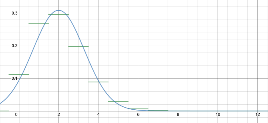
First, in this section, I want to explain the graphical interpretation. To make this easier to draw, let me use a smaller n. Suppose that we are rolling n=12 dice, and that a “success” is rolling a six. I want to calculate the probability of rolling either 1, 2, or 3 sixes. If S is the number of sixes, then
$$P(1\leq S\leq 3) = P(S=1) + P(S=2) + P(S=3).$$
Now,
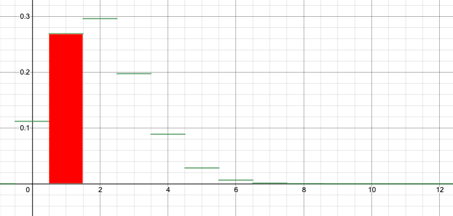
$$P(S=1)=b(1;12,1/6)=\binom{12}{1}\left(\frac{1}{6}\right)^1\left(\frac{5}{6}\right)^{12}\doteq 0.2692,$$
and that is the height of the bar of the graph at $k=x=1$. The width of the bar is 1, so I can think of 0.2692 as the area of the bar.
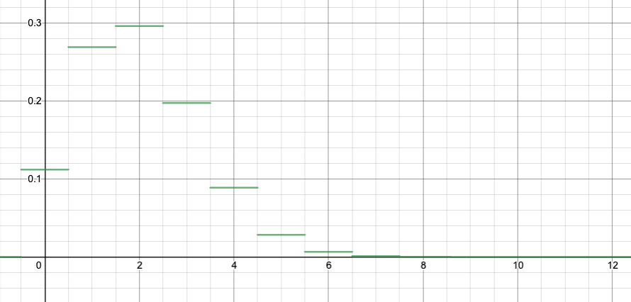
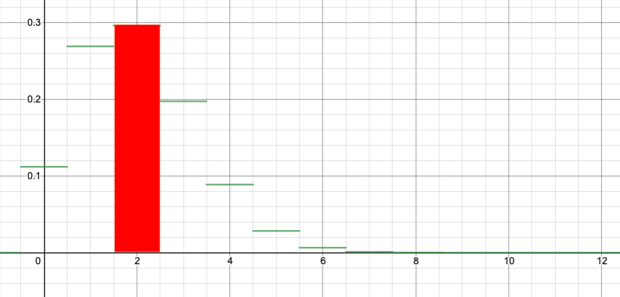

You can see in this way that computing the probability for a range of values for the binomial distribution is converted to the problem of computing an area.
To see how the normal approximation would help, let’s superimpose the normal approximation on this graph:
If we can compute the area under the normal curve from x=0.5 to x=3.5, that should approximate the area of the red rectangles above. (Recall that I’ve arranged it so the bar for the binomial k=1 goes from x=0.5 to x=1.5, and so on.)
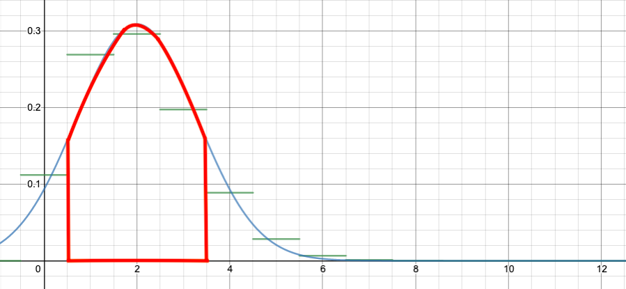
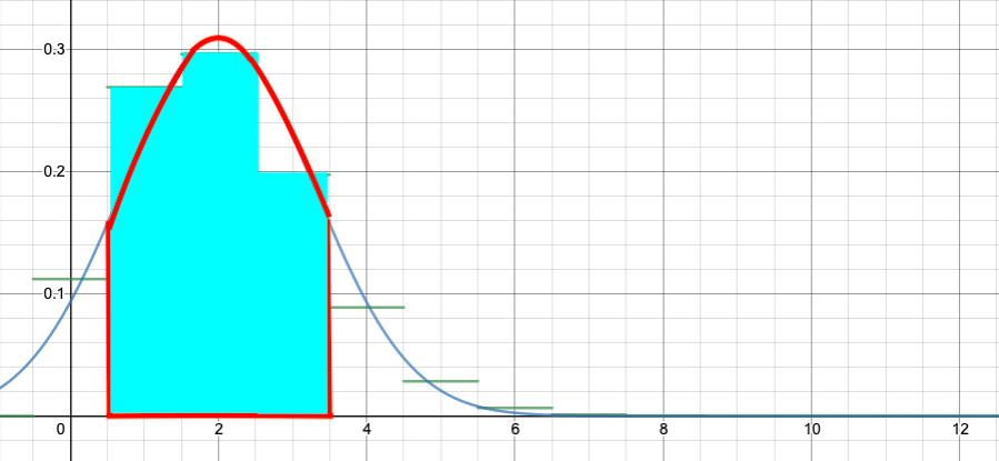
Looking at the graph, the approximation is only OK. But for that problem, it would have been easy to just add $b(1,12,1/6)+b(2,12,1/6)+b(3,12,1/6)$. The approximation becomes better—and more necessary—for larger n.
For example, let’s go back to our example of flipping 100 coins. We want to find the probability of between 40 and 60 heads. This would have taken a tedious addition. But by the same logic as above, that probability is approximately equal to the following area:

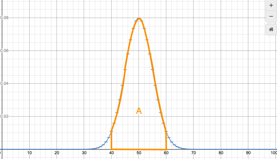
So, if we can calculate the area of regions under the normal curve, then we can use that to calculate probabilities for the variable k in the binomial distribution to lie in a certain range.
I’ll tell you how to calculate those areas in a moment. First I want to make a more general comment, then I need to introduce one more idea, then we will get back to calculating this area.
3. Probabilities for ranges in a continuous distribution
Before we go on with the approximation to the binomial distribution, I want to make an important point.
It is often the case that we are making measurements of something that (at least theoretically) varies continuously. The number of heads we get flipping 100 coins is always a whole number. However, if we measure people’s heights, or length of a bolt, or time waiting for a computer error, or time to a radioactive decay, or mass of a particle, then those measurements don’t come in natural discrete bits. Of course we will only be able to measure them to a finite number of decimal places; but, at least in theory, these measurements are represented with continuous, real numbers, rather than discrete integers.
If that is the case, then the probability of any exact result is actually zero! It never happens that we wait exactly 1 second for a radioactive decay, or that a person is exactly 72 inches tall. What we would actually measure is something like, the decay took 1.000 seconds, up to an experimental error of +/-0.003 seconds. If we could somehow measure perfectly accurately, it is impossible that the decay took 1.000000….. seconds with infinitely many zeroes.
For continuous variables, the only probabilities that make sense are probabilities for ranges. It does make sense to say that we waited between 0.995 and 1.005 seconds for a decay. It does make sense to ask, what is the probability we need to wait between 1 and 3 seconds?
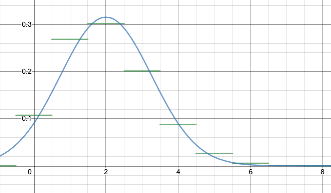
In that case, we use an argument similar to what we said above about the binomial distribution, though in the other direction. Suppose, for example, that we are measuring people’s heights. We approximate the continuous distribution of heights with a discrete one; we break heights into ranges of, say, inches, and for each one-inch range we graph the probability of someone falling in that range. But that is only approximating the theoretically continuous heights. We could make a better approximation by breaking heights into half-inches, and making twice as many bars, one for each half-inch range, and graphing the probability of falling into each half-inch range.
We run into a technical problem if we continue this way: the probability of having the height fall into a smaller and smaller range also gets smaller and smaller. The height of the graph goes to zero everywhere! To avoid this, we must instead graph the probability density: the probability of a person falling in a certain range, in probability per inch. For example, if 6% of people fall into the 64 to 64.5 inch range, and 10% of people fall into the 64.5 to 65 inch range, then overall 16% of people fall in the one-inch range from 64 to 65 inches. We would record this as a probability density of 12% per inch in the 64 to 64.5 inch range, and 20% per inch in the 64.5 to 65 inch range, for an average of 16% per inch in the 64 to 65 inch range.
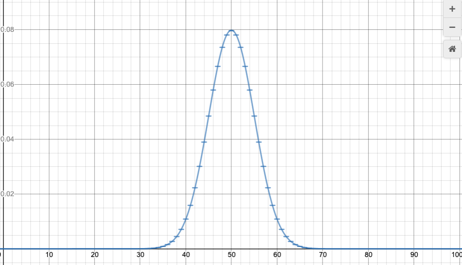
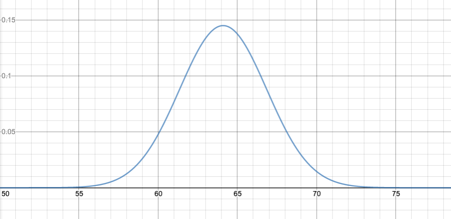
In the limit, we end up with a continuous graph. The normal distribution is an example of a continuous graph. As an example, heights of women ages 20–29 in the US, in a national survey from 1994, were found to be closely approximated by a normal distribution, with $\mu=64.1$ inches and $\sigma=2.75$ inches:
The advantage of graphing probability densities is that, if we want the probability in some range, it will equal the area under the graph.
(More generally, what we need is a way of assigning a probability to every event—that is, to every reasonable subset of your sample space. Such a rule is called a measure, and the general formalism of how to do this is called measure theory. For continuous variables, this is rather fancy mathematics in general, which is why we aren’t covering it. A graduate course in probability—and Volume II of our textbook—would spend a lot of time working out the fundamentals of measure theory for this reason. We will keep it simple, intuitive, and not totally rigorous.)
For example, in the graph I just showed, the actual probability density in the 64 to 65 inch range appears to be between 0.140 and 0.145 per inch. So if I want to know how many people fall in that range, I would multiply the one-inch range by about 0.143 per inch, gives me about 14.3% or so of people in that range.
If I wanted to know how many people fell into the 60 to 65 inch range, I could repeat that calculation for the 60 to 61 inch range, the 61 to 62 inch range, and so on, and add the results.
I could get a more accurate answer by subdividing into smaller parts. For example, for the 64 to 65 inch range, I could say that probability density is about 0.144 per inch for the 64 to 64.5 inch range; that gives me 0.072, or 7.2% of the population in that range; I could say it is about 0.140 per inch for the 64.5 to 65 inch range, so that gives me 0.070, or 7.0% of the population in that range; in total, I get about 14.2% of the population in the 64 to 65 inch range.
In all these cases, I am computing the area under the graph for the range of interest. This is what a continuous probability distribution means: you compute probabilities from it by finding the area under it, for the range in question.
Calculus has a concept for that, called the integral, and written with $\int$ (a long “S”, standing for a “continuous Sum”). If $f(x)$ is the continuous probability distribution, we would write what I just said as follows:
$$P(a\leq x\leq b) = \int_a^b f(x)\,\mathrm{d}x.$$
In words, the probability that x is in the range from a to b is the area under the graph of f(x) from a to b.
In the case of the normal probability distribution, this would read
$$P(a\leq x\leq b) = \int_a^b \frac{1}{\sigma\sqrt{2\pi}}e^{-\frac{1}{2}\left(\frac{x-\mu}{\sigma}\right)^2}\,\mathrm{d}x.$$
Now, if you haven’t taken any calculus, then this doesn’t mean much; all I’ve done is introduced a symbolic notation meaning “find the area under the graph from x=a to x=b“. Which is actually pretty much true.
If you have taken any calculus, you know there are methods for working these things out. You may be tempted to try to figure this out right now. Just find the antiderivative! And then you can figure it out!
Unfortunately, it is not possible to find the antiderivative of that formula in elementary functions (rational functions of polynomials, exponentials, logs, and trig functions). The antiderivative function exists—but there is no formula for it in terms of our standard functions.
If you haven’t taken any calculus, this talk of antiderivatives won’t make sense, but don’t worry, they don’t help much here anyway.
What do exist are very efficient and accurate computer methods for finding an integral (=an area under a given curve), even if you can’t find it exactly by calculus trickery.
To apply these, I first want to standardize things a bit.
4. Z-scores
A Z-score is a way of transforming a normal distribution to a standard one. First let me state the result, then I’ll explain it.
Suppose that x is some variable with a normal probability distribution $N(x;\mu,\sigma)$. (By that I mean, that, for any a and b, $$P(a\leq x\leq b)=\int_a^bN(x;\mu,\sigma)\,\mathrm{d}x.$$ Define a new variable $$Z=\frac{x-\mu}{\sigma}$$. Then the new variable sigma has a probability distribution of the “standard” normal distribution, $N(x;0,1)$.
The variable Z is often called a “Z-score”. Its meaning in words is: how far is x from the mean $\mu$, measured in standard distributions $\sigma$? Recall that $\sigma$ measures, roughly, the “width” of the distribution, so the value of Z is saying, how far is x from the center of the distribution, measured relative to how wide the distribution is.
That was kind of vague. Let me give you some examples.
Example: Suppose that we are flipping n=100 coins. Then the binomial distribution $b(k;100,1/2)$ is well-approximated by a normal distribution, with mean $\mu=np=50$ and standard deviation $\sigma=\sqrt{npq}=5$.
(i) Getting k=70 heads corresponds to a Z-score of $Z=\frac{70-50}{5}=4$. You can say this in words as “70 is 4 standard deviations above the mean”. This is quite far from the center, as measured by the “width” of the distribution, and is therefore quite unlikely.
(ii) Getting k=45 heads corresponds to a Z-score of $Z=\frac{45-50}{5}=-1$. That is, 45 is 1 standard deviation below the mean. This is more likely.
(iii) Getting k=50 heads corresponds to a Z-score of $Z=\frac{50-50}{5}=0$. That is, 50 is the mean, so it is a distance of 0 standard deviations from the mean.
To continue the example, let’s say we want to calclulate the probability of getting 60 or fewer heads on the 100 coins. This would be computed by the binomial distribution,
$$P(h\leq 60)=b(0;100,1/2)+b(1;100,1/2)+b(2;100,1/2) +\dotsb+b(60;100,1/2)$$
or
$$P(h \leq 60) = \binom{100}{0}\left(\frac{1}{2}\right)^{100} + \binom{100}{1}\left(\frac{1}{2}\right)^{100} +\binom{100}{2}\left(\frac{1}{2}\right)^{100} + \dotsb + \binom{100}{60}\left(\frac{1}{2}\right)^{100}.$$
This would be a very tedious calculation.
The probability is equal to the area of all the bars under the binomial distribution graph, from k=0 up to k=60. This gives us a picture, but doesn’t help calculate it yet.
However, the binomial distribution can be approximated by the normal distribution:
$$b(x;100,1/2) \approx N(x;50,5),$$
so
$$P(0\leq x\leq 60) \approx \int_{-0.5}^{60.5} N(x;50,5)\,\mathrm{d}x.$$
Note that I am going up to 60.5, because the bar for 60 on the discrete binomial distribution graph would stretch between 59.5 and 60.5. Similarly, the bar for 0 goes from -0.5 to 0.5.
This is better; a computer could do this for you. However, it is even better to standardize. The value x=60.5 corresponds to Z=2.1. The value x=-0.5 corresponds to Z=-10.1. And the Z-score is normally distributed with mean $\mu=0$ and standard deviation $\sigma=1$. So
$$P(x\leq 60) =P(Z\leq 2) \approx \int_{-10.1}^{2.1} N(x;0,1)\,\mathrm{d}x.$$
The advantage here is that we can always use areas under the standard normal curve $N(x;0,1)$; so we can make one standard computer program, or one standard set of tables, and that will work for all problems.
There is another standard choice: the area is tabulated starting from $-\infty$ up to $x$. So, the standard cumulative normal distribution is
$$\Phi(x)=\int_{-\infty}^{x}N(x;0,1)\,\mathrm{d}x.$$
The function $\Phi(x)$ is a standard function in computer algebra systems like Wolfram Alpha. You can find online calculators which will give you $\Phi(x)$, or areas under the standard normal curve more generally; here is a typical one.
I don’t understand why $\Phi(x)$ is not a standard function on calculators or calculator apps. Scientific calculators and calculator apps have a lot of fancy functions now, but usually not this common and frequently used function, for some reason.
More classically, the function $\Phi(x)$ is tabulated in standard tables; there is a table like this in the text, Chapter VII, Table 1, pages 176–177:
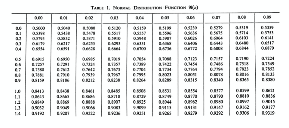
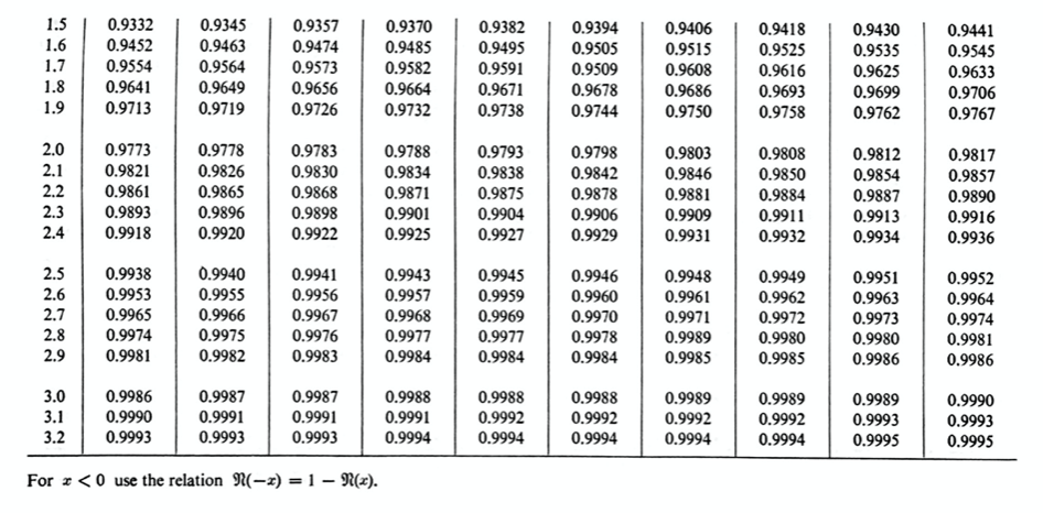
People still use these tables; you can still find them in standard statistics textbooks (perhaps because they are not offered on most calculators).
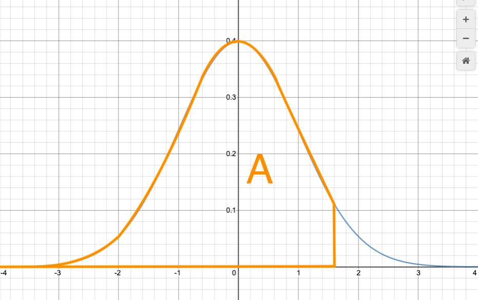
To give an example of how to use the table, let’s find the area A that I showed in the graph above. I said it was $\Phi(1.6)$. Looking on the table, this value is approximately 0.9452. For another example, from the table, $\Phi(1.64)$ would equal 0.9495.
Example: Back to the question of flipping 100 coins, and finding the probability that 60 or fewer are heads. We found that
$$P(h\leq 60) =P(Z\leq 2) \approx \int_{-10.1}^{2.1} N(x;0,1)\,\mathrm{d}x.$$
The area below Z=-10.1 is totally negligible, so we can replace the -10.1 with a $-\infty$. Therefore, $P(h\leq 60) =P(Z\leq 2.1) \approx \Phi(2.1)$, and from the table, $\Phi(2.1)\doteq 0.9821$. There is about a 98.2% chance that the number of heads will be 60 or fewer.
Example: When flipping 100 coins, what is the probability $P(40\leq h\leq 60)$?
This will be approximated by
$$P(40\leq h\leq 60)\approx \int_{-39.5}^{60.5}N(x;50,5)\,\mathrm{d}x.$$
Converting to Z-scores,
$$P(40\leq h\leq 60)\approx \int_{-2.1}^{2.1}N(x;0,1)\,\mathrm{d}x.$$
Now, note that $N(x;0,1)$ is symmetric around x=0. Also note that $\Phi(0)=0.50$ (because the total area under $N(x;0,1)$ must be 1, the probability of anything happening). So
$$\int_{0}^{2.1}N(x;0,1)\,\mathrm{d}x=\Phi(2.1)-0.5\doteq 0.4821.$$
(Draw the pictures of the areas to see what I am doing there!)
Also by the symmetry,
$$\int_{-2.1}^{0}N(x;0,1)\,\mathrm{d}x=\int_{0}^{2.1}N(x;0,1)\,\mathrm{d}x\doteq0.4821$$
as well, (again, draw the picture!), so
$$P(40\leq h\leq 60)\approx \int_{-2.1}^{2.1}N(x;0,1)\,\mathrm{d}x \doteq 0.4821 + 0.4821 = 0.9642$$
There is about a 96.4% chance that the number of heads appearing is between 40 and 60.
Exercise 1:
(a) Suppose that we flip a coin 1000 times. What is the probability that the number of heads is between 450 and 550?
(b) Suppose that we flip a coin 200 times. What is the probability of getting more than 120 heads?
(c) Suppose that we roll a die 50 times. What is the probability of getting more than 12 sixes?
6. The normal distribution for its own sake
The normal distribution is not only relevant as an approximation to the binomial distribution. It happens very frequently in mathematics, science, and other applications. There are a number of reasons for its universality, not of all I will be able to explain in this class, though I will mention one at the end of this lecture.
For this reason, it will be helpful to remember some general features of the normal distribution. Here are what I think are some of the most important points.
- The normal distribution is NOT just “a bell curve”. It is a bell curve of a very particular exponential form.
- The tails decrease very rapidly, even faster than exponentially. The chance of being more than 6 standard deviations away from the mean ($Z\geq 6$ or $Z\leq-6$) is basically zero for all practical purposes.
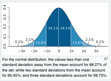
- There is about a 68% probability of being within 1 standard deviation of the mean ($-1\leq Z\leq 1$).
- There is about a 95% probability of being within 2 standard deviations of the mean ($-2\leq Z\leq 2$).
- There is about a 99.7% probability of being within 3 standard deviations of the mean ($-3\leq Z\leq 3$).
There is a lot more to say about the normal distribution, but we won’t have time to get to much more in this class.
7. Relative standard deviation of the binomial distribution
The fact that the standard deviation of the binomial distribution is
$$\sigma=\sqrt{npq},$$
combined with the rules of thumb about the normal distribution, can give you some useful quick estimates.
For example, if we flip a coin 100 times, $\sigma=5$. So, roughly, 68% of the time, there will be between 45 and 55 heads, and 95% of the time there will be between 40 and 50 heads.
If we flip a coin 1000 times, $\sigma\doteq 15.811\approx 16$, so roughly, 68% of the time there will be between 484 and 516 heads, and 95% of the time there will be between 468 and 532 heads.
Note that, percentage-wise, the number of heads is much more likely to be close to the mean with 1000 coin flips than with 100. This is true in general: the binomial distribution gets relatively narrower as n gets bigger.
If we think of the standard deviation $\sigma$ as a proportion of $n$, we find
$$\frac{\sigma}{n}=\frac{\sqrt{npq}}{n}=\frac{\sqrt{pq}}{\sqrt{n}}.$$
The percentage-wise “breadth” of the peak is inversely proportional to $\sqrt{n}$. If n gets four times as big, the peak becomes two times thinner, percentage-wise.
If we flip a coin 1,000,000 times, then $\sigma=500$, so 95% of the time, the number of heads will be between 499,000 and 501,000. The variation from the expected number 500,000 of heads is no more than 1,000/500,000=0.2%, with a probability of 95%.
When you are presented with a situation that is modeled by a binomial distribution, computing $\sigma=\sqrt{npq}$ can give you a quick, intuitive sense of how much variation you would typically expect to see away from the mean.
Exercise 2: Suppose that people are voting for party A with an unknown probability p. We are trying to estimate p by means of polling. Suppose we survey 1000 people, and a of the people say they will vote for party A. (Assume perfect response rate, perfect honesty, etc.) We therefore estimate the probability of people voting for party A to be a/1000.
How far off from the true value of p is our estimate a/1000 likely to be? (First, think of exactly how this is a situation where the binomial distribution applies. Then, determine a range in which the value of a is, say, 95% likely to lie. This range, divided by 1000, is what we would call our 95% confidence interval for our estimate of p.
8. The central limit theorem
I can only give a rough idea of this theorem now. I can give a more precise formulation after we do Chapter IX. We won’t have time to prove it. But it’s an important enough concept that I want to mention it.
In the case of the binomial distribution, we can imagine that we are running an experiment n times, and each time the experiment has a “success”, it records a 1, otherwise it records a 0. Then the number of successes is the sum of the results of all n experiments. We have seen that this number of successes has a probability distribution that is approximately the normal distribution. That is, each time we run the n experiments, we will get a different number of total successes; different values of that number will have different probabilities, and tabulating those probabilities will approximately give a normal distribution, with $\mu=np$ and $\sigma=\sqrt{npq}$.
We could imagine something more complicated than just a 0 or 1 result. For example, if we are measuring some animals and trying to get their average weight, then we are measuring the individual weights (which vary randomly), taking the sum, and then dividing by their number. We could then ask, over different samples of animals, how will this average weight vary? What will be the probability distribution? This will be an important question if we want to know how much confidence to put in our average weight: how off is it likely to be from the “true” average, given our sample size?
Similarly, we could imagine that we have a server which takes requests for data. In any given minute, it is taking requests from n different sources, and each source has an amount of data it requests each minute, which varies randomly. We could then ask, how is the total data requested going to vary from one minute to the next? What is the probability distribution for the total amount of data requested per minute?
The central limit theorem says: under very general conditions, as long as the different experiments are independent, then, no matter how else they are varying randomly, when we sum their results, we get a normal distribution. This is very broadly applicable and useful.
For example, it says that in almost all cases, if our sources of measurement error are independent, then the distribution of measurement errors in an experiment will always be normal.
It says that, in an example like the server example above, when we have a whole lot of random influences coming together to create a total, provided the influences are independent, the sum of those random influences will vary randomly according to a normal distribution.
We can even say more about the standard deviation of that normal distribution. For example, when we are weighing the animals, this will give us a way of estimating our confidence in our final measurement of the average weight. However, that will have to wait until after Chapter IX.
Conclusion
This has been a marathon! I hope it has been helpful. I hope you’re not too exhausted. I am! This 7 week (actually 6 week!) pace is hard for math.
You may want to take a look at Chapters VII and X, to get a sense of how they are organized, and what they contain. I wouldn’t recommend trying to read them very carefully at this time, but if you can get a general sense of them, it may help you orient yourself with respect to the book.
I haven’t asked many exercises in this lecture. There will be more problems in the corresponding assignment.
After that, next up is random variables and expectation, Chapter IX. That will complete the core concepts of probability theory (at least as far as this course is concerned); the rest of the class will be on applying the concepts to more examples.