OK, let’s begin reading the book!
What I will do in this first lecture is give you a guide to the reading, section by section. (All the readings are from the Feller textbook, a link to which is on the main page.)
I will intentionally NOT be explaining things here which are explained in the text. The intention is for you mainly to be learning from the book.
I’m going to be very detailed, because I’m trying to give my suggestions about how to read a book like this, as explicitly as I can. In future lectures, I’ll gradually be less detailed about the reading, and talk more just about the math. But I will assume that you are reading the later chapters in the same detailed way.
For each section, I recommend looking at my initial suggestions, then reading the section of the text, then coming back and reading my other suggestions or questions. Then move on to the next section. (But of course you can do this in any order you find useful!)
Preamble Assignment #1, which I sent you before the term, was intended to set you up for this chapter and assignment. Hopefully it was helpful. However, if you haven’t done PA#1 already, I would suggest not doing it now, and just diving in to Chapter I. Everything we need about sets is covered in Chapter 1, so if you understand everything in the Chapter, you do not need to go back and complete the PA#1. If you are finding the material on sets in Chapter 1 confusing and would like more explanation, you could go back and look at PA#1 and the reference book I suggested there.
(Preamble Assignments #2, 3, and 4 will not be used in Chapters I or V; they will be important when we get to Chapter VI. If you haven’t done the PA already, I’d suggest working on them now whenever you find time, so that you are ready for Chapter VI when we get there.)
Prefaces and Note
(Pages vii–xii.)(Page numbers refer to the numbers on the actual pages, NOT the page numbers of the pdf.)
Usually it is worthwhile to skim over the preface and initial notes for a book. The author is going to make notes for potential instructors, which won’t necessarily make sense to you, so you shouldn’t read super-carefully. However, it can be helpful to give some context for the book
Introduction: The Nature of Probability Theory
(Pages 1–6.) (Page numbers refer to the numbers on the actual pages, NOT the page numbers of the pdf.)
Usually it is a good idea to read the introduction to a text, without reading it too carefully. That is the case here.
The author is making some general comments about the nature of the subject, and the book’s approach to it. This can be quite helpful to start you thinking about the subject.
I would suggest keeping brief notes—maybe a few words or a sentence for each paragraph. If questions occur to you, jot them down.
Since this is an overall statement of approach and philosophy, there are probably points here that won’t make much sense until you’ve seen some more examples. So it isn’t worth working very hard to totally understand every statement. However, recording some observations or questions to come back to later can help set you up for what is to come.
Exercise 1: Which statement in this chapter seemed most interesting to you? Which statement seemed the most confusing? Make a note of these for discussion later.
Chapter I: The Sample Space
I.1. The Empirical Background
(Pages 7–9.)
Before reading
Take a glance over the section you are about to read. It is about three pages. The next section is “examples”, which means that this section must be setting up the stage, and maybe defining some important terms.
It will be important to start reading carefully now. Read slowly. Keep notes as you are reading. Try to make a note of the important points in each paragraph, even if it is just scattered words to remind yourself later.
OK, read the section, then come back and we will compare notes!
. . .
OK, are you back? Don’t worry if it took a while, reading math is slow.
Let’s compare notes.
First paragraph (page 7)
What did you take away as the most important point here? Mine was the last sentence of the paragraph: that the author is aiming to describe the possible results of an experiment or observation.
When you are given a list of examples like this, it is often a good idea to adopt one or two examples yourself, which you like. These can be your pet examples. For example, I chose as my pet example experiments:
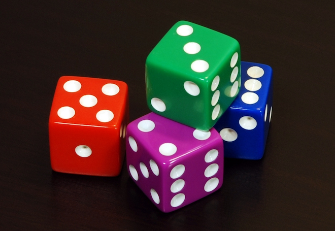
a) rolling one die (a nice simple example)
b) rolling two dice (a slightly more complicated example).
Then, as I read ahead, I imagine those examples for any abstract definition, and I see if I can apply anything the author introduces to my particular examples.
Exercise 2: Come up with a couple of pet examples of your own. I would suggest one that is very simple, and one that is a little more complicated. Apply each concept that follows to your pet examples.
Second and third paragraph (pages 7–8)
The author is talking here about the distinction between the real world, and an idealized mathematical model. That will be something to keep in mind as we go forward. Did you have questions here? If so, you should bring them up in class or on the Slack.
Fourth paragraph (page 8, starting with “For uniform terminology…”)
The author is explaining the term event. It will be important to make a note of every definition or explanation of new terminology. It can be helpful to apply any new concept to your personal pet examples. Here are the examples I came up with for “event”:
a) rolling one die and the number comes up a “1”
b) rolling one die and the number comes up even (either 2, 4, or 6)
c) rolling two dice and they both come up 6
d) rolling two dice and they come up a 1 and a 2
e) rolling two dice and they both come up even
f) rolling two dice and they add to 6
Exercise 3:
a) Come up with a few more examples of “events” for rolling one or two dice.
b) Come up with some examples of “events” for your choice of pet example experiments.
Also, be sure to make sure you understand the definitions of “bridge” and “poker” in the footnote. You don’t need to know how to play these games, just what is stated in text. Ask in class or on Slack if it isn’t clear.
Fifth paragraph (pages 8–9, starting “We shall distinguish..”)
First of all, check that you understand the author’s examples, by recreating them yourself if possible.
Is it clear to you why the event “sum six” for two dice corresponds to five simple events? There is a tricky point here that is worth noticing. I won’t say what it is now, but ask in class if you don’t see it (or if you don’t agree that it should be five simple events).
List all the simple events for “two odd faces”, and see if you get nine of them, as the author says.
Then, try to apply the terms to your choice of experiments:
Exercise 4:
a) For each of my examples of “event” I listed above (for rolling one or two dice), say whether the event is compound or simple. If it is compound, list the simple events that it decomposes into.
b) For your examples of “event” that you listed in the previous exercise, say whether the event is compound or simple. If the event is compound, list the simple events that it decomposes into.
Sixth paragraph (page 9, starting “If we want to speak…”)
In your notes, list the terms you need to remember. Then apply those terms to your examples:
Exercise 5:
a) For my example experiments (of rolling one die, or rolling two dice), what are the “sample points”, and what is the “sample space”? How many points are in the sample space in each of these two examples?
b) In your example experiments, what are the “sample points”, and what is the “sample space”? How many points are in each of your sample spaces?
I.2. Examples
(Pages 9–13).
Before reading
Three things I would note.
One: this is a long section. You might want to read part, then come back to these suggestions, or write notes and think a bit, then come back to reading more.
Two: There are concrete examples in this section. You should always treat examples as if they were solved exercises. Try to work out as much as you can of each example on your own, and compare to what the author writes, to gain practice and check your understanding.
Three: There appear to be many variants on one example. When there’s a long list, it might be good to understand a couple of items, and then flag the rest to come back to later. You don’t always have to read in order, as long as you get to everything eventually.
(a) Distribution of three balls in three cells
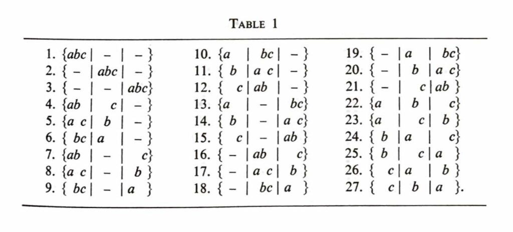
First paragraph: You should see the author’s statement, and Table 1, as a solved exercise. That is, you should try to solve it yourself, pretending you don’t see the answer in Table 1; and then compare your answer to the author’s. This is the best way to check your understanding, and to internalize the ideas. To be more specific:
Exercise 6:
a) Can you think of a reason why there would be 27 possible ways to place three balls into three cells (or boxes)? (Try thinking about how many choices you have at each step. Ask about this in class if you aren’t sure.)
b) Make your own list of all the ways to put three balls into three boxes. Try to make the list yourself, without referring to Table 1, and see if you can get all 27 possibilities. (This maybe seems redundant to you, since Table 1 is right there. But working this through yourself will help you thoroughly understand this important example.) You’ll have to come up with a bit of a system, in order to avoid accidentally missing any possibilities. Having done this, when you look back at Table 1, can you see what the author’s system was?
Second paragraph: This is a sequence of definitions of events, and statements about those events. Check each statement carefully yourself, and make sure that you agree with the author’s claim in each case. If anything is confusing, try to isolate what you disagree with or don’t understand. If you can’t resolve the difficulty, make a note of it to return to later, and/or to ask in class. Do not leave anything unresolved!
(b) Random placement of r balls in n cells
First paragraph (page 10)
Exercise 7: a) The author claims that for r=4 balls and n=3 cells, the sample space contains 64 points. Can you calculate this yourself?
b) Similarly, for r=n=10, the author claims there are 10^(10) sample points; can you check this?
c) These two examples are too long to list out all the sample points. It might be worthwhile to pick a smaller r and n, other than r=n=3, and to list all the sample points, similar to Table 1. Try that for at least one other choice of r and n. Do more if it is interesting!
d) That brings up an important point: it can often be helpful to work out the very simplest examples. What happens if r=1 and n=1? What if r=1 and n is anything? What if n=1 and r is anything? What would the next simplest examples be, and what happens in those cases?
Second paragraph (page 10, starting “We use…”)
What point is he trying to make in this paragraph?
List of examples (b,1) through (b,16) (pages 10–11)
It might be a good idea to read a few of these examples carefully, and skim the rest. I would recommend reading the first two or three carefully, picking one more that interests you to read carefully, and then just read over the rest without worrying too much about understanding.
(Though if you are up to it, go ahead and read them all carefully! I am just making the point that you don’t always have to read strictly in order.)
I’ll just make notes on the ones I chose to read carefully:
(b,1) Birthdays: This is an interesting mental model for thinking about probability problems on birthdays. Sometimes having a different mental picture (one ball for each person, placing the ball in one of 365 boxes) can help you think about the problem differently. (For these questions, ignore leap days; that is, ignore the possibility of a February 29 birthday.)
Exercise 8:
a) Suppose we have r people, and the experiment we are doing is recording their birthdays. How many sample points are there (as a formula in r)?
b) Suppose we have 2 people. How many sample points are there? Let A be the event that the two people have the same birthday. How many sample points are in A? Can you determine from this what the probability of A is? Is it what you would have guessed?
c) Suppose we have 366 people. What do we know for sure about them?
d) Sometimes it is helpful to start thinking about problems you can’t solve yet. For example, the next question I would be inclined to ask myself is: with 3 people, what is the probability that two of them have the same birthday? Think about how you would solve this a bit. You don’t have to find an answer now. But any partial progress you make on the question will help set you up for when the author starts to introduce more techniques. (And if you can solve it now, nice work! Try 4 people!)
(b,2) Accidents: This example made me realize something: up until now, I had been assuming that all sample points are equally probable. However, this example makes it clear that this doesn’t need to be true.
For example, you could say there is r=1 accident, being placed in n=7 boxes for one of the 7 days. There would be 7 sample points. But there is no reason they would be equally likely. If you know anyone who has worked in a hospital, you know that accidents happen more often on Fridays and Saturdays.
If there are r=2 accidents, being placed in n=7 boxes for one of the 7 days, then there are going to be 7 x 7 = 49 sample points, just as we worked out before, and we could (in principle) list them like before. But their probabilities would all be different.
I mention this just to illustrate that, as you read, you might realize that you misunderstood something before, or that you made incorrect assumptions, and you have to go back and correct them. That is a normal part of the process!
(b,3) Firing at targets: OK, I’m imagining something like “skee-ball” here.
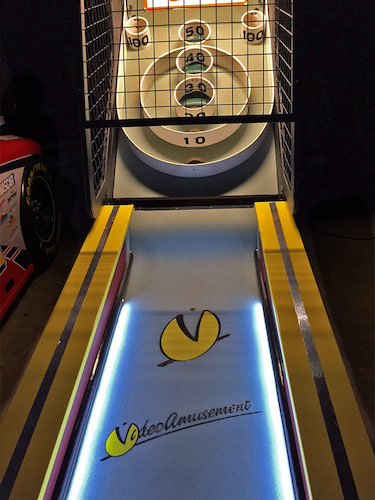
So again, not all targets are equally likely! But that’s OK, we are just listing possibilities. In this pictured game, there are 7 “boxes” (actually holes the ball can go into), which have been assigned 0,10,20,30,40,50,100, and 100 points. If I throw 10 balls, there are 7^(10) possible outcomes, though certainly not all equally likely!
I am also realizing that the examples are a little repetitive now. The examples are intended to illustrate that many different practical examples may be represented with the same abstract model, of placing “balls” into “cells”. So I’m reading a little less carefully.
(b,8) Dice: I look at this example a bit more carefully, because dice were my pet example.
Let me try r=1. Then the statement is that throwing 1 die is the same as placing a ball randomly in one of six boxes. That makes sense!
Exercise 9:
a) Think about what this example means when r=2. Does the placing of 2 balls into boxes actually correspond correctly with the throwing of 2 dice? Do you get the same number of points in the sample space? What does the analogue of Table 1 look like? (You don’t have to write out every entry, but write out enough to convince yourself that you can if you need to.)
b) Let A be the event that the two dice show the same number. Can you use this model to find the probability that this happens?
c) You may have been thinking about this already, so I will mention it here: does it matter which die is which? (If that hasn’t worried you yet, read on, we’ll come back to this question.)
I won’t make comments about the other examples, but I encourage you to read the ones you find interesting, and bring up any questions or comments in class.
(c) The case of indistinguishable balls
First Paragraph and Table 2 (pages 11–12)
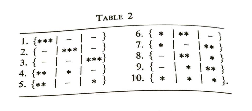
As before, you should treat an example as a solved exercise:
Exercise 10: Work out all the possibilities for putting 3 indistinguishable balls into 3 cells. I would recommend doing this two ways:
a) Go through Table 1, and identify all the entries that are now considered the same (this is how the author explains it);
b) Start again fresh, listing all possibilities you can think of for placing three balls in three cells, but now not distinguishing which ball is which. Again, you will need some sort of system to keep it straight. When you have your answer, look again at Table 2, and try to guess what system the author has used.
Exercise 11: For this new sample space, assuming the balls are randomly placed, are all the sample points going to have the same probabilities? Why or why not? If not, what are the probabilities? (Your answers to this may depend on how you interpret “randomly placed”… In any case, this will be useful to think about.
Exercise 12: Here is a question I asked myself at this point. Could I have figured out that there would be 10 sample points, without listing them all out? A little earlier, the author gave examples of different numbers r of balls and n of cells. For example, we figured out the number of sample points when r=4 and n=3, and also when r=n=10, when the balls were considered distinguishable, without listing all possibilities. Now that the balls are considered indistinguishable, can I do this? Can you figure out how many sample points there are in those cases, without listing everything? (Let me emphasize that I did NOT know how to answer this question at this point. It is good to be asking yourself questions: this starts you thinking, and sets you up for what is coming next. And it was helpful to me to think about how to solve this problem, so I recommend trying it for a bit. I would suggest starting with small r and n examples, where you can check your answers by listing out possibilities. I don’t expect that you will be able to find a complete answer now, but that is OK, working on it will be worthwhile! Don’t drive yourself crazy though!)
Second paragraph (page 12, beginning “Whether or not…“)
Note that whether we are thinking about the balls as distinguishable will depend on the questions we are asking. But which way we treat a problem shouldn’t change the final answer.
Third paragraph (page 12, beginning “In the scheme above…”)
The author says that if the cells are considered indistinguishable, then the sample space only has three points. Convince yourself that this is in fact true! Again, the author is saying, it doesn’t matter if we can really tell the boxes apart; the question is whether we are worried about which box is which or not, for the purposes of our problem.
Exercise 13: At this point, a question occurred to me. The author has treated the cases:
(i) balls distinguishable, cells distinguishable
(ii) balls indistinguishable, cells distinguishable
(iii) balls indistinguishable, cells indistinguishable
What about the case of
(iv) balls distinguishable, cells indistinguishable ?
Does this even make sense? If so, can you list all the possibilities, like in Table 1 and Table 2? How many sample points do you get?
In the exercise above, note that I am making two points. One, I would like you to think about the question I asked. But two, maybe more importantly, I would like you to be thinking of your own questions as you are reading. This habit of asking questions is, I think, one of the main ways to get better at reading mathematical texts.
(I have also now learned that “distinguishable” sounds weird if you say it enough times.)
(d) Sampling (pages 12–13)
Does this make sense to you? Make notes if not!
Note that the author is assuming in this example that we only care about the total number of smokers. What if we cared about some other information about them? Oh, wait, now I’m looking at the next section…
(e) Sampling (continued) (page 13)
It’s nice when you ask a question, and then the author goes on to answer it in the next paragraph!
Does this all make sense? As I was reading, I thought, “Can the numbers M_s, F_s, M_n, F_n be anything? What are the restrictions on them? Are they independent of each other?”. But then the author seems to have answered my questions in the next sentence.
The author says there are 176,851 sample points. I thought for a bit about how I might figure this out. But I ended up not spending too long on that question, because it seemed to me that (a) this seemed hard, and (b) it seemed like a special example, and maybe not like it would be super important (unlike the balls and cells examples, which seemed more universal).
That’s just a guess at this point. I want to make the point here that it is good to ask yourself questions, and to try to check everything the author says; BUT it can get overwhelming if you take it too far. So it’s OK to leave some things to be understood later. I just made a note of this question to myself, and hoped it would get explained later.
It is a bit of a judgment call about which questions you follow up, and how long you spend doing so. Making that judgment is part of the skill of reading a text like this. If you just read lightly, and don’t work out any examples or ask yourself any questions, you will rapidly feel like you aren’t understanding anything (or you will get to the exercises and not be able to solve any). On the other hand, if you get too obsessed about answering every point before continuing, it will feel overwhelming and take you too long to finish. Sometimes it is OK to take something for granted, and maybe come back to it later.
(f) Coin tossing (page 13)
Hopefully this all makes sense at this point. Make a note to yourself if not.
(g) Ages of a couple (page 13)
My apologies for the assumption that every couple is heterosexual!
Note that every pair of ages corresponds to a pair of numbers, which corresponds to a point in a plane (referred to an x-y coordinate system). Therefore, this sample space may be represented as a set of points in the plane.
The author doesn’t specify whether we are thinking of the ages as discrete or continuous. That is, whether someone can be 39.56 years old, or if they are counted as 39 years old until their 40th birthday. If the ages are discrete, then the sample space is a finite set of dots in the plane. If the ages are continuous, then the sample space is a continuous region in the plane, consisting of infinitely many points.
It may be worthwhile to draw the pictures that the author is describing, to make sure that you understand the statements.
(h) Phase space
When the author refers to something you don’t know about, you can safely skip over it! Here, he seems to be making this point for those people who have studied statistical mechanics, to refer it to something that they know.
I know that I’ve been saying you should try to understand everything thoroughly, but it can also be a good idea to know when to skip something. It would not be very worthwhile to go to wikipedia and try to learn about “statistical mechanics” and “phase spaces”, because this seems to just be a tangential point.
(Of course, sometimes you decide to skip over something, and then later it turns out to be important, and you have to revisit it; that is fine!)
Intermission
Phew, this is exhausting, right?

I’m surprised at how long it is taking me to write all this out. I am describing all the thought processes that I went through when reading the chapter.
It is making me aware of just how much I’m doing when I’m reading a mathematical text. I hope that it is helpful to you to make this all explicit. I will do this in progressively less detail as we go on to future chapters.
OK, let’s get back to it!
3. The Sample Space. Events.
Before reading
Take a quick look at the section. Now that that author has given some examples, he is going on to make some formal definitions. It will be a good idea to write out a list of the terms you need to know as you are reading. It will also be a good idea to try to apply the terms to examples you have seen already (including your pet examples).
On the other hand, it is also a good idea not to get too hung up on totally understanding definitions on a first reading. Sometimes the definitions only become clear when you start to see how they are used. So it is OK to feel at this point like it isn’t totally clear, and to read ahead and then come back.
First paragraph (pages 13–14)
Apply the definitions to some of the examples you have done: for example, for rolling two dice, think about what the sample space is, what the sample points are, and what some events are. Or do the same for the balls in cells.
Note that the word “aggregate” is a synonym of the word “set”. (They mean the same mathematically, but some authors switch back and forth, just for variety.)
Second paragraph (“Example” on page 14)
Again, treat this like a solved exercise. Check every statement that the author makes, writing it out yourself if necessary.
Last paragraphs (page 14)
To make it clear: the author is saying that a sample space is by definition a mathematical set. This is why I assigned some reading on sets in Preamble Assignment #1.
A set is a collection of objects, or elements, or points (those words are taken to be synonymous).
By definition, two sets are equal if, and only if, they have the same elements, or points. That means that a set does not come with any ordering of its points; if you list the points in a different order, it is still the same set. Also, there cannot be repetition in a set; a point is either in a set or is not in a set. A point cannot be repeated multiple times in a set (you could do so, but we would think of it as the same set with the point listed once).
(If we wanted to consider lists where the order mattered, or repetition mattered, we could do that. Those mathematical concepts have different names, instead of “sets”.)
An event is a subset of the sample space. A set A is a subset of a set S if every point in A is also in S.
4. Relations Among Events
Before reading
Look ahead: the author is now introducing some formal language and symbolism. The author is abstracting the examples. In order to keep your bearings, it will be good to keep a pet example in mind. Every time the author introduces a new abstract concept, apply it to your pet example, to keep everything concrete in your mind.
First paragraph (pages 14–15)
The weird-looking $\mathfrak{S}$ is an “S” in German “Fraktur” font, standing for “Sample space”. This font is sometimes used for math symbols.
Note that the symbol “$\in$” is supposed to be a stylized “e”, standing for “is an element of”. The word “element” is more common now than “point”, though both are used. They are synonymous.
Definition 1 (page 15)
The symbol “$\emptyset$” is now more common than “0” for the empty set. The symbol “0” for the empty set emphasizes the analogies between set theory and arithmetic (we’ll see that more later).
I am using my pet examples of “rolling one die” or “rolling two dice”. The examples of empty set events I came up with were “I roll one (normal) die and it comes up 7”, or “I roll two dice and the sum of the two dice is 1”.
You should come up with your own examples for each definition (it can help to stick to one pet example).
Definition 2, and the rest of page 15
Exercise 14: For your pet examples, make examples for the definitions as follows. In each case, make sure that you understand the events both in words and in lists of outcomes. (For example: one of the examples I came up with was rolling one die; I made the event A to be “rolling a 3 or greater”, so it consisted of {3,4,5,6}; then A’ was “rolling less than a 3”, so it consisted of {1,2}.)
a) Come up with a couple of examples of events A, and find their complements A’.
b) Come up with a couple of examples of pairs of events A and B, and find the events AB (they both occur) and $A\cup B$ (either A or B or both occur).
c) Come up with an example of a pair of events A and B, such that $AB=\emptyset$.
d) Come up with an example of a pair of events A and B, such that $AB’=\emptyset$. Do the same for $A’B’=\emptyset$.
Note that it is nowadays more common to write the intersection of A and B as $A\cap B$, rather than AB. The notation AB emphasizes some analogies to arithmetic, and it also works nicely sometimes for probabilities, as we will see later.
Definition 3 (page 16)
Exercise 15: As before, make some examples for the definitions. Be sure to understand the events both in words, and in lists of outcomes.
a) Come up with an example of three events A, B, and C, and find the intersection ABC and the union $A\cup B\cup C$.
b) Come up with an example of three events A, B, and C which are mutually exclusive.
c) Come up with an example of three events A, B, and C which satisfy $ABC=\emptyset$, but A, B, and C are not mutually exclusive. Try to explain the difference between “$ABC=\emptyset$” and “A, B, and C are not mutually exclusive” to yourself in words, if you can.
Definition 4, and the preceding paragraph (page 16)
The author is saying that the statement “event A implies event B” (or, equivalently, “if A occurs then B occurs”), can be translated into set theory language as “event A is a subset of event B“.
This is a little tricky to get used to. It will help to invent some examples, as the author suggests. It will also help to draw some diagrams like Figures 1 and 2 on page 15. (These are called “Venn diagrams”.)
Exercise 16:
a) Come up with a couple of real-life examples of $A\subset B$. Say each example in words in two ways: that “if condition A holds then condition B holds”, and “the set of things satisfying condition A is a subset of the set of things satisfying condition B“.
b) For your pet example, come up with two events A and B such that $A\subset B$, and express the relationship between events A and B in words.
c) Take a look back at Figures 1 and 2 on page 15, and make sure you understand the examples the author gives there. Draw a diagram that represents $A\subset B$. Go back and think of your examples in (a) and (b) pictorially in this way.
The diagrams can be quite helpful in imagining the meaning of different expressions.
Exercise 17:
a) Copy Figure 1 on page 15, and label every region with symbol (for example, ABC’, etc.). (There should be eight regions to label in total.)
b) Make up some expressions in A, B, and C, and shade them in on diagrams like Figure 1 on page 15. For example, try expressions like $(A\cup B)C’$, or $A’\cup B’\cup C’$.
Note: in many texts, $B-A$ is defined to be $BA’$ always; note that this book defines $B-A$ to be $BA’$ only when $A\subset B$. Note also that many books now use the symbol $B\setminus A$ rather than $B-A$.
Examples (pages 16–17)
I found these examples helpful in clarifying the definitions.
As before, treat every example like a solved exercise. Every time the author makes a statement, work it out yourself.
Exercise 18: Check all the examples on pages 16–17 yourself. Draw a Venn diagram whenever it makes sense. Make note of anything where you can’t see how to check the author’s statement, or if you get a different answer than the author.
5. Discrete Sample Spaces
On a first reading, I found the title of this chapter confusing. As far as I understood, every example we have had so far of a sample space has been discrete! So why this title now?
As I started to read, I realized that the author is introducing infinite sample spaces in this chapter. Every sample space up until now has been finite, that is, every sample space has had finitely many points.
The author is NOT introducing continuous infinite sample spaces. For example, a length or a weight could have any decimal value in a certain range, so the sample space would be an interval in the real numbers. Continuous sample spaces are much trickier. (He devotes a whole second volume to them!) So what he means with the title of this chapter is really “Infinite discrete sample spaces”.
Aside: This is a standard way of talking in mathematics, that can occasionally be confusing. (I even got confused by it this time!) One uses a word that is less restrictive (“discrete” rather than “finite”) in order to add possibilities.
For example, suppose I had a formula I wanted to explain for whole positive numbers first, and then to explain it for negative whole numbers next. It might make most sense to name the chapters “whole positive numbers” and then “negative numbers”. But mathematicians would often name those chapters “whole positive numbers” and then “integers”—because integers include the whole positive numbers plus the negative numbers.
Anyway, back to probability.
Example (a) (pages 17–18)
Note that there are infinitely many points in this sample space. However, almost all the points are represented by a finite string of T and H. That is because, by definition, we agreed to stop flipping the coin as soon as an H appears. So his E_1, E_2, E_3, etc are the only possibilities (right?).
The only infinite string is if a head (somehow) never comes up. So E_0 could be represented as TTTTT… going infinitely far.
Example (b) (page 18)

It took me a few tries to understand this example correctly. I had to re-read what the author wrote carefully. Then I imagined three actual people I know as players a, b, and c, and I talked myself through it, writing down and diagramming as I went.
“So, a and b play. Maybe a wins the first time, or maybe b. If a wins the first time, then in the second game, a plays c. If a wins, then the tournament is over. Aha, that is what ‘aa’ means! OK, now if c wins the second game…”
Exercise 19: Talk this through with yourself or a friend, and convince yourself that he has indeed listed all the possibilities of the sample space.
If you still can’t figure it out, make a note to bring it up with other students or in class.
Definition and last paragraph (page 18)
I don’t have anything to add here, but if it isn’t all clear, please make a note to ask!
6. Probabilities in Discrete Sample Spaces
OK! We were wondering before about how probabilities were assigned—in particular, if every point in the sample space had to have the same probability. Now the author is going to talk about it. Good.
If you glance ahead a little, you will see that in this chapter, he is talking about the empirical idea, and giving examples. Then in the next chapter, he is giving the formal mathematical definitions.
Personally, I find it very helpful to glance ahead and back like this as I am reading. It helps me to know what the purpose of this chapter is, and where I am in the whole voyage.
By the way, the title is again perhaps a little confusing: “discrete” means either discrete and finite, or discrete and infinite.
First three paragraphs (pages 19–20)
The author is making some philosophical remarks here.
The author’s main point seems to be to make the distinction between an idealized mathematical model and a physical scenario. No real coin flips H and T with exactly probability 1/2 each. But it is simpler to make an idealized mathematical model in which the probabilities are exactly 1/2. Then our model will apply to reality, to the extent that its assumptions are reflected in the real situation.
(And as I mentioned in the introductory lecture, even if a real coin did flip H or T with probability exactly 1/2 each, how would we ever know? We could only ever do finite sequences of flips. In a finite sequence, the number of H and T is not going to be exactly 1/2, even if the coin is exactly fair. In fact, if it was always exactly 1/2, that would be very suspicious!)
Secondarily, the author is hinting at some of the difficult philosophical problems we talked about in the introductory lecture. What does a probability of an actual event mean, anyway?
He seems to be bringing this up to say, we don’t need to answer these philosophical questions, in order to have an agreement about the mathematical axiomatic definition of a probability, which he will proceed to describe in the next chapter.
Example (a) (page 20)
If we pick balls out of a bucket one at a time, and for each ball, make a random choice of the cell to put it in, then all 27 points of the sample space in Table 1 will have the same probability, of 1/27.
Now, the “balls” may not be literal balls; they may represent any of the situations in the examples on pages 10–11, among other things. So equal probabilities may or may not be a good model.
Exercise 20: Look at the examples (b,1)–(b,16) on pages 10–11, and try to decide which ones make sense to assign equal probabilities to all points in the sample space on Table 1. (In particular, the author suggests that this does not make sense for (b,1), (b,7), or (b,11); can you see why?)
Example (b) (pages 20–21)
Note that if we don’t distinguish the balls—if they all look the same—then we could paint them red, green, and blue, and it wouldn’t change the experiment. So if we randomly select a cell for each ball as described above, then the probabilities for Table 1 are all equal, which means the probabilities for Table 2 are not equal.
Exercise 21: Under the above assumptions, find the probabilities of each of the possibilities in Table 2. (The author gives the answer on p.20; work it out yourself and then check against his answer.)
However, if the assumptions are different, then the probabilities could be different.
Amazingly, there is a physical situation where all the points of the sample space in Table 2 have equal probabilities. This is the “Bose-Einstein” statistics the author mentions, which applies to identical spin-zero particles, like photons. This makes photons more likely to “clump together” than if they were randomly distributed in the most intuitively sensible way. This is called a “Bose-Einstein condensate”.
Neither the author nor I is expecting you to understand that statement! He is just making the point that the probabilities may be assigned in a non-obvious way, (and making the connection to physics for those who have studied it, or will study it).
Example (c) (pages 21–22)
As I said in the introductory lecture, the number of heads in 100 coin tosses is not going to be always 50—it would be suspicious if it were! But it should average to 50, presumably. And it shouldn’t vary from 50 “too far”, at least not “too often”. How much is “too far” and “too often”? That’s what we want to answer soon!
The story of the book “A Million Random Digits” by RAND corporation is actually quite interesting! And the Amazon reviews are funny…
7. The Basic Definitions and Rules
Looking over it, this is another chapter with formal definitions (and even a Theorem).
As before, you should do two things:
(i) Be sure to make a note of each concept (even just listing the names, so you remember what you need to remember); and
(ii) For every abstract definition or theorem, come up with an example (which you could choose from your running pet examples, and/or the examples in the book).
I will collect all my suggestions, for examples you should be making, in the following exercise. But hopefully you are getting into the habit of doing this automatically by now!
Exercise 22:
a) For the “fundamental convention”, give an example in which the probabilities aren’t all equal. (For my example, I took the experiment as “rolling two dice and taking the sum”. The sample space then consists of the numbers 2, 3, 4, …, 12. I worked out the probabilities of each of these numbers, and checked that they added to 1. You can do that one if you like, or you can pick your own.)
b) Can you think of an example where there is a point in a sample space whose probability should be zero? (There was at least one example in the earlier sections.)
c) Think of an example where we have already used the Definition on page 22: where we had an event A which is compound, and found its probability P{A} by adding the probabilities of all the sample points in A. (Or make up a new example.)
d) In equation (7.3) on page 22, the author says that $$P(A_1\cup A_2)\leq P(A_1)+P(A_2).$$ (i) Come up with an example where the left side is strictly less than the right side; (ii) come up with an example where the two sides are equal.
e) Use a few examples to check that the Theorem on the bottom of page 22 does in fact give the correct probability of $A_1\cup A_2$.
f) Work through the example on page 23.
Conclusion
Whew, we’re done! Finally!
Before you go on to the exercises, take a moment now to do one more thing. Having reached the end of the chapter, you should go back and make a summary for yourself.
A good summary should be very short. It can just be a list of the sections in the chapter, and a list of what topics or important facts were in them; or you can organize it your own way. (I never feel I really understand something until I reorganize it in a way that makes most sense to me.)
OK, now you’re really done reading the chapter! Congratulations! Pat yourself on the back. Get a snack. Take a breather before you dive into the next thing, which is the Chapter I assignment!