
In this lecture, I will return to the Markov chain that I introduced in the previous lecture. I want to provide answers for some of the questions I asked you there, particularly about finding an equilibrium state. But I also want to go further and show how to simplify the evolution, using eigenvectors. In the process, I will connect back to the material we have been doing on dual vectors and projections.
The example Markov chain from last time
Let me remind you of the example from last time. I had a system of agents that could be in two states, 1 or 2. I start with $x_1(0)$ agents in state 1, and $x_2(0)$ agents in state 2. In each time step, some agents would change states, summarized by the following graph:
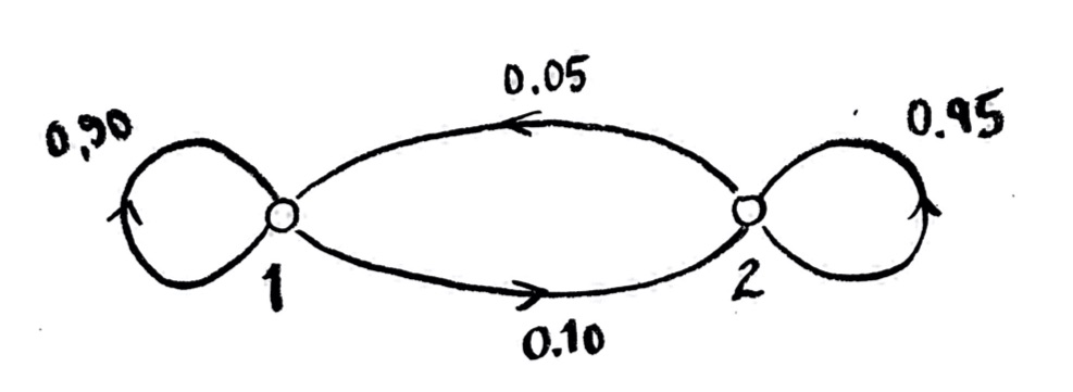
In each time step, $0.10$ of the agents in state 1 would switch to state 2, and $0.05$ of the agents in state 2 would switch to state 1.
Alternately, this can model only one agent, or system, which changes states with some probabilities. Then $x_1(t)$ and $x_2(t)$ are the probabilities of the single system being in state 1 or 2 respectively.
The goal is to understand, as completely as possible, the behavior of $x_1(t)$ and $x_2(t)$ as functions of time.
The evolution equations we set up last time
In the last lecture, we set up the evolution equation. It is:
$\begin{bmatrix}x_1\\x_2\end{bmatrix}(t+1)=T\begin{bmatrix}x_1\\x_2\end{bmatrix}(t)$,
where the transition matrix $T$ for this system is
$T=\begin{bmatrix}0.90&0.05\\0.10&0.95\end{bmatrix}$.
Alternatively, we can write the evolution equation in terms of differences. The change from time step $t$ to $t+1$,
$\Delta\begin{bmatrix}x_1\\x_2\end{bmatrix}(t):=\begin{bmatrix}x_1\\x_2\end{bmatrix}(t+1)-\begin{bmatrix}x_1\\x_2\end{bmatrix}(t)$,
is given by
$\Delta\begin{bmatrix}x_1\\x_2\end{bmatrix}(t)=\Delta\begin{bmatrix}x_1\\x_2\end{bmatrix}(t)$.
Oops, that equation looks silly, doesn’t it!? It’s because I have two clashing notations here (which are totally standard, so I don’t want to change them). The greek capital Delta, “$\Delta$”, on the left refers to “change in the vector”. But the same symbol $\Delta$ on the right refers to what is called the weighted graph Laplacian matrix,
$\Delta=\begin{bmatrix}-0.10&0.05\\0.10&-0.05\end{bmatrix}$,
which is multiplied by the vector.
Anyway, that means that, for each time step $t$,
$\begin{bmatrix}x_1\\x_2\end{bmatrix}(t+1)=\begin{bmatrix}x_1\\x_2\end{bmatrix}(t)+\Delta\begin{bmatrix}x_1\\x_2\end{bmatrix}(t)$,
which means
$\begin{bmatrix}x_1\\x_2\end{bmatrix}(t+1)=(I+\Delta)\begin{bmatrix}x_1\\x_2\end{bmatrix}(t)$,
where $I=\begin{bmatrix}1&0\\0&1\end{bmatrix}$. There are some advantages to writing it both ways.
Finding the steady state
The first question I asked is, does this system approach an equilibrium state? If I start with $x_1(0)$ agents in state 1, and $x_2(0)$ agents in state 2, will the number of agents $x_1(t)$ and $x_2(t)$ settle down over time, or will they oscillate (or even jump around chaotically?). And if they do settle down, what will the equilibrium values be, and how will they depend on the initial values $x_1(t)$ and $x_2(t)$?
We can say that we are looking for possible vectors $\begin{bmatrix}x_1\\x_2\end{bmatrix}$ with the property that
$T\begin{bmatrix}x_1\\x_2\end{bmatrix}=\begin{bmatrix}x_1\\x_2\end{bmatrix}$;
so the transition from time step $t$ to $t+1$ doesn’t change the values.
This is connected to the eigenvectors I talked about in the previous lecture. Such a vector would be an eigenvector for the matrix $T$, with eigenvalue of 1.
We could set this up as linear equations and solve. But there is a trick which makes it a little easier. If I write $T=I+\Delta$, then a steady state vector would have the property that it doesn’t change under the evolution equation. So we’re looking for possible vectors $\begin{bmatrix}x_1\\x_2\end{bmatrix}$ with the property that
$\Delta\begin{bmatrix}x_1\\x_2\end{bmatrix}=\begin{bmatrix}0\\0\end{bmatrix}$.
That is, the vectors we are looking for are eigenvectors of the matrix $\Delta$ as well, with eigenvalue 0. (Note that my definition of eigenvector requires that the vector be non-zero. The zero vector would satisfy this equation, but wouldn’t be very helpful.)
Another word for this is that the vector $\begin{bmatrix}x_1\\x_2\end{bmatrix}$ is in the kernel of matrix $\Delta$. I’ll have more to say about kernels soon.
Anyway, the system $\Delta\vec{x}=\vec{0}$ is a little easier to solve.
Understanding exercise: computing the steady-state vectors
a) Solve the system $\Delta\vec{x}=\vec{0}$.
b) Check that your solutions are in fact eigenvectors of $\Delta$, with eigenvalue $0$.
c) Check that your solutions are in fact eigenvectors of $T$ as well, with eigenvalue $1$.
d) Can you explain why, practically for this model, that any multiple of a steady state vector is also a steady state vector? (A rough explanation is fine.)
e) Suppose that $A:V\to V$ is any linear transformation, and $\vec{v}\in V$ is an eigenvector of $A$ with eigenvalue $\lambda$. Prove that then, for any non-zero scalar $a$, the vector $a\vec{v}$ is also an eigenvector of $A$, with eigenvalue $\lambda$.
f) Suppose that the initial state is $x_1(0)=100$ and $x_2(0)=0$. Find the steady state that this would approach to.
g) Find the steady state vector, in terms of any given $x_1(0)$ and $x_2(0)$.
h) If the system is interpreted as a single agent, moving between states 1 and 2 with some probabilities, then what are the steady-state probabilities?
You should find that the solution set to $\Delta\vec{x}=\vec{0}$ is
$\left\lbrace\begin{bmatrix}x_1\\x_2\end{bmatrix}:\begin{bmatrix}x_1\\x_2\end{bmatrix}=s\begin{bmatrix}1\\2\end{bmatrix},\,s\in\mathbb{R}\right\rbrace$.
Any non-zero scalar multiple of the vector $\begin{bmatrix}1\\2\end{bmatrix}$ will be an eigenvector of $\Delta$ with eigenvalue $0$, and also an eigenvector of $T=I+\Delta$ with eigenvalue $1$. These are the possible steady states.
If we know the initial numbers of agents $x_1(t)$ and $x_2(t)$, then we can solve for the unknown scalar as well. The trick is that, as I noted last time, this system preserves total number of agents (or preserves probability, if we think of it as a single agent). (There are various names for this condition. In our current context, such a system is called Markov. In physics, it says that this satisfies the continuity equation, or is incompressible.)
Anyhoo, since I know the number of agents is constant over time, the variable
${x’}_1 = x_1+x_2$
is constant in time. Consequently, the steady-state vector will have to satisfy two equations:
$\begin{bmatrix}x_1\\x_2\end{bmatrix}=s\begin{bmatrix}1\\2\end{bmatrix}$, and $x_1+x_2=x_1(0)+x_2(0)$.
Understanding exercise: computing the specific steady-state vector
Solve the above equations, to find the parameter $s$ and therefore the specific steady-state vector.
We obtain for the steady-state vector
$\begin{bmatrix}x_1\\x_2\end{bmatrix}=\dfrac{x_1(0)+x_2(0)}{3}\begin{bmatrix}1\\2\end{bmatrix}$,
or, absorbing the 1/3 into the vector,
$\begin{bmatrix}x_1\\x_2\end{bmatrix}=\left(x_1(0)+x_2(0)\right)\begin{bmatrix}\frac{1}{3}\\\frac{2}{3}\end{bmatrix}$.
If we interpret the model as a single agent, and interpret $x_1(t)$ and $x_2(t)$ as probabilities, then $x_1(0)+x_2(0)=1$, so the steady-state probabilities are
$\begin{bmatrix}x_1\\x_2\end{bmatrix}=\begin{bmatrix}\frac{1}{3}\\\frac{2}{3}\end{bmatrix}$.
In summary: it seems that, no matter where the system starts, that long-term, 1/3 of the agents end up in state 1, and 2/3 of the agents end up in state 2. Or, if it is a single agent, it will keep jumping back and forth, but it will spend 1/3 of the time in state 1, and 2/3 of the time in state 2.
Long-term behavior more precisely
But wait, that’s not really a total answer. We have identified an equilibrium state: if the system is exactly in that state, it will stay there. But will it get there? And will it stay there if it is not exactly in the state? Think of a ball at the very peak of a smooth hill: if it is exactly at the peak, it is in equilibrium and will stay there. But it will almost never end up there from other initial conditions; and if it is slightly away from the peak, it will move away.
If you did the computer experiments, or if you think about the meaning of the model, it should be pretty plausible that the system always moves toward the equilibrium that we identified. Using the machinery of eigenvectors and eigenvalues, we can show that more precisely, and also say exactly how it is moving toward equilibrium. (This analysis will be important in many other areas as well, not just this problem.)
We have already identified one eigenvector of $T$ and $Delta$, the vector
$\begin{bmatrix}\frac{1}{3}\\\frac{2}{3}\end{bmatrix}$,
with eigenvalue 1 for $T$, and eigenvalue 0 for $\Delta$.
I’ll tell you soon how to find another eigenvector for $T$ and $\Delta$. For the moment, I just want to show you how you can use the other eigenvector to compute the evolution easily.
So, let me pull the other eigenvector that I computed earlier out of the oven:

I claim that the vector
$\begin{bmatrix}1\\-1\end{bmatrix}$
is an eigenvector of both $T$ and $\Delta$.
Understanding exercise:
Check this claim, and find the corresponding eigenvalue.
Again, I’ll tell you how I cooked up this vector later. But for the moment, let me show you how I can use it. I’m going to use it two ways:
- I can make a basis out of eigenvectors, and T will be simple in that basis; or
- using dual eigenvectors, I can write T as a sum of projection operators, which puts it in a simple form.
Eigenvalue basis
Here’s the trick of the first method: make a basis (coordinate system) out of the eigenvectors of $T$! This basis will be nicely adapted to expressing the matrix $T$.
So, let $B’=\{{\vec{e}’}_1,{\vec{e}’}_2\}$ be the basis consisting of vectors
${\vec{e}’}_1=\begin{bmatrix}\frac{1}{3}\\\frac{2}{3}\end{bmatrix}$, ${\vec{e}’}_2=\begin{bmatrix}1\\-1\end{bmatrix}$.
Any vector $\vec{v}$ can be uniquely expressed as a linear combination of vectors this basis. I’m going to call the corresponding coefficients the coordinates $x_1’$ and $x_2’$ of the vector $\vec{v}$:
$\vec{v}=x_1\vec{e}_1+x_2\vec{e}_2=x’_1{\vec{e}’}_1+x’_2{\vec{e}’}_2$.
The operators $T$ and $\Delta$ operate very simply on this basis:
$T\left(x_1’\vec{e}_1’+x_2’\vec{e}_2’\right)=x_1’T\left(\vec{e}_1’\right)+x_2’T\left(\vec{e}_2’\right)=\lambda_1x_1’\vec{e}_1’+\lambda_2x_2’\vec{e}_2’$.
All it does is stretch in the $\vec{e}_1’$ direction by the eigenvalue $\lambda_1$, and in the $\vec{e}_2’$ direction by eigenvalue $\lambda_2$. So, if we express $T$ in the basis $B’$,
$T\begin{bmatrix}{x’}_1\\{x’}_2\end{bmatrix}_{B’}=\begin{bmatrix}\lambda_1&0\\0&\lambda_2\end{bmatrix}_{B’}\begin{bmatrix}{x’}_1\\{x’}_2\end{bmatrix}$.
We know that $\lambda_1=1$ and $\lambda_2=0.85$. So, in the basis of eigenvectors, $T$ is represented very simply as a diagonal matrix,
$[T]_{B’}=\begin{bmatrix}1&0\\0&0.85\end{bmatrix}_{B’}$.
In this form, $T$ is quite simple and easy to work with. For example, if you wanted to find the state after 13 time steps, you’d just have to find
$T^{13}\begin{bmatrix}{x’}_1(0)\\{x’}_2(0)\end{bmatrix}_{B’}=\begin{bmatrix}1&0\\0&0.85\end{bmatrix}^{13}_{B’}\begin{bmatrix}{x’}_1(0)\\{x’}_2(0)\end{bmatrix}_{B’}=\begin{bmatrix}1^{13}&0\\0&(0.85)^{13}\end{bmatrix}\begin{bmatrix}x’_1(0)\\x’_2(0)\end{bmatrix}_{B’}$.
No need to do thirteen matrix multiplications!
But, I’m not given the initial data in the $x’_1$, $x’_2$ coordinates, and I don’t want the answer in those weird coordinates either. So I need to change coordinates.
Change of coordinates for a vector: concrete linear equation version
Let’s see how to do this in a concrete way. We’ll make it more systematic in the next section.
Let’s suppose we have initial values $x_1(0)=40$ and $x_2(0)=20$.
Understanding exercise: Change of basis by linear equations
With the initial value vector $\vec{v}(0)=\begin{bmatrix}x_1(0)\\x_2(0)\end{bmatrix}=\begin{bmatrix}40\\20\end{bmatrix}$, find the initial values of the primed coordinates, $x’_1(0)$ and $x’_2(0)$.
Here’s the solution to the exercise above. By the definitions above,
$\begin{bmatrix}x_1(0)\\x_2(0)\end{bmatrix}=\begin{bmatrix}40\\20\end{bmatrix}=x’_1(0){\vec{e}’}_1+x’_2(0){\vec{e}’}_2=x’_1(0)\left(\begin{bmatrix}\frac{1}{3}\\\frac{2}{3}\end{bmatrix}\right)+x’_2(0)\left(\begin{bmatrix}1\\-1\end{bmatrix}\right)$,
so we get the linear equations
$\frac{1}{3}x’_1(0) + x’_2(0)=40$
$\frac{2}{3}x’_1(0) – x’_2(0)=20$.
These have the unique solution $x’_1(0)=60$, $x’_2(0)=20$.
Using eigenbasis to compute transformation
Understanding exercise: Computing powers of T in the eigenbasis
Suppose again that we have starting conditions $x_1(0)=40$ and $x_2(0)=20$.
a) Use the previous exercise to find a simple expression for $x_1(n)$ and $x_2(n)$ for any positive integer $n$.
b) Optional computing exercise: use the expression to make a table of $x_1(n)$ and $x_2(n)$ for $n=1,2,\dotsc,20$.
c) Use the expression to find $x_1(20)$ and $x_2(20)$.
d) Use the expression to find the limit of $x_1(n)$ and $x_2(n)$ as $n$ gets large.
Here’s the solution to the previous exercise. We have
$\begin{bmatrix}x_1\\x_2\end{bmatrix}(1)=T\begin{bmatrix}x_1\\x_2\end{bmatrix}(0)=T\begin{bmatrix}40\\20\end{bmatrix}=T\left((60)\begin{bmatrix}\frac{1}{3}\\\frac{2}{3}\end{bmatrix}+20\begin{bmatrix}1\\-1\end{bmatrix}\right)$
$=(60)T\begin{bmatrix}\frac{1}{3}\\\frac{2}{3}\end{bmatrix}+(20)T\begin{bmatrix}1\\-1\end{bmatrix}=(60)\begin{bmatrix}\frac{1}{3}\\\frac{2}{3}\end{bmatrix}+(20)(0.85)\begin{bmatrix}1\\-1\end{bmatrix}$.
So in the same way, we get
$\begin{bmatrix}x_1\\x_2\end{bmatrix}(2)=T^2\begin{bmatrix}x_1\\x_2\end{bmatrix}(0)=(60)\begin{bmatrix}\frac{1}{3}\\\frac{2}{3}\end{bmatrix}+(20)(0.85)^2\begin{bmatrix}1\\-1\end{bmatrix}$
and so
$\begin{bmatrix}x_1\\x_2\end{bmatrix}(n)=T^n\begin{bmatrix}x_1\\x_2\end{bmatrix}(0)=(60)\begin{bmatrix}\frac{1}{3}\\\frac{2}{3}\end{bmatrix}+(20)(0.85)^n\begin{bmatrix}1\\-1\end{bmatrix}$.
Putting in numbers, we have
$\begin{bmatrix}x_1\\x_2\end{bmatrix}(20)\doteq(60)\begin{bmatrix}\frac{1}{3}\\\frac{2}{3}\end{bmatrix}+(0.775)\begin{bmatrix}1\\-1\end{bmatrix}=\begin{bmatrix}20.775\\39.225\end{bmatrix}$.
In the limit as $n\to\infty$, we have $(0.85)^n\to 0$, and hence the limiting state is $\begin{bmatrix}20\\40\end{bmatrix}$, as we had predicted in the previous section.
Change of coordinates for a vector: systematic matrix version
Let’s do this a little more systematically.
In this section, I’ll work through how to change coordinates for a vector, from the old standard basis to the new basis of eigenvectors. This isn’t specific to this example; it works for any change of basis in a finite-dimensional vector space.
Let
$S=\begin{bmatrix}\frac{1}{3} & 1 \\ \frac{2}{3} & -1\end{bmatrix}$.
I have made the columns of this matrix equal to the new basis vectors, the eigenvectors ${\vec{e}’}_1$ and ${\vec{e}’}_2$. This matrix $S$ has the effect of converting from $x’_1$, $x’_2$ coordinates to the $x_1$, $x_2$ coordinates, because
$S[\vec{v}]_{B’}=S\begin{bmatrix}x’_1\\x’_2\end{bmatrix}=x’_1\begin{bmatrix}\frac{1}{3}\\\frac{2}{3}\end{bmatrix}_{B} + x’_2\begin{bmatrix}1\\-1\end{bmatrix}_B=[x’_1{\vec{e}’}_1+x’_2{\vec{e}’}_2]_B=[\vec{v}]_B$.
Understanding exercise: Change of basis matrix
The logic of that previous equation is important. Let’s check it by trying some examples.
a) Suppose that we start with the vector $\vec{v}={\vec{e}’}_1=(1){\vec{e}’}_1+(0){\vec{e}’}_2$, so that $x’_1=1$, $x’_2=0$, and $[\vec{v}]_{B’}=\begin{bmatrix}1\\0\end{bmatrix}_{B’}$. Check that multiplying this vector $[\vec{v}]_{B’}$ times $S$ gives the vector $[\vec{v}]_{B}$.
b) Do the same thing with the vector $\vec{v}={\vec{e}’}_2$.
c) Think through the logic again of the equation above. (I don’t have anything particular for you to write for this part. This is one of those things in math where you need to do the incantation to yourself about a hundred times before it sticks. . . )
This means that the matrix $S^{-1}$, if it exists, converts from $x_1$, $x_2$ coordinates to $x’_1$, $x’_2$ coordinates. Explicitly:
$S[\vec{v}]_{B’}=[\vec{v}]_{B}$
$S^{-1}S[\vec{v}]_{B’}=S^{-1}[\vec{v}]_{B}$
$I[\vec{v}]_{B’}=S^{-1}[\vec{v}]_{B}$
$[\vec{v}]_{B’}=S^{-1}[\vec{v}]_{B}$
So, to summarize,
$[\vec{v}]_{B}=S[\vec{v}]_{B’}$
$[\vec{v}]_{B’}=S^{-1}[\vec{v}]_{B}$
These are the change of basis equations, which apply for changing coordinates of vectors between any two bases $B$ and $B’$. The matrix $S$ is always defined by having columns equal to the $B’$ basis vectors, written in the $B$ coordinates (i.e., the columns are the coefficients of the $B’$ basis vectors, when they are written as linear combinations of the $B$ basis vectors).
We’ll talk about matrix inverses more generally soon, but for the moment you might want to recall that the inverse of a $2\times 2$ matrix is given by
$\begin{bmatrix}a&b\\c&d\end{bmatrix}^{-1}=\dfrac{1}{ad-bc}\begin{bmatrix}d&-b\\-c&a\end{bmatrix}$.
Understanding exercise: Change of basis example
Use this procedure to redo a previous exercise: show how to write the vector $\begin{bmatrix}40\\20\end{bmatrix}_{B}$ in the $B’$ coordinate system. Check that you get the same answer as before.
Next, I want to use this change of coordinates of vectors, to change coordinates for the transformation $T$.
Change of basis for a linear transformation
Now I want to change basis for the transformation $T$. This is the same thing we did earlier, but I want to do it in matrix form now, rather than as linear equations. This method will apply for any linear transformation $A:V\to V$, from a finite-dimensional vector space to itself. (It also applies to $A:V\to W$ between two different vector spaces, with minor modifications.)
First of all, we know that, in the standard basis $B$, the matrix of $T$ is
$[T]_B=\begin{bmatrix}0.90 & 0.05 \\ 0.10 & 0.95\end{bmatrix}_B$.
We can find $[T]_{B’}$ one of two ways. First, we can change coordinates by means of the matrix $S$. This works conceptually as follows:
- $[T]_{B’}$ expects an input in the $B’$ basis, while $[T]_B$ expects an input in the $B$ basis. $[T]_{B’}$ will output its answer in the $B’$ basis, while $[T]_B$ will output its answer in the standard $B$ basis.
- So, to create $[T]_{B’}$, we need to first take an input in $B’$ coordinates, and then convert it to $B$ coordinates, using $S$.
- Then we have the vector in $B$ coordinates, so $[T]_B$ happily eats it, and spits out its answer, also in $B$ coordinates.
- Since we are looking for the answer in $B’$ coordinates, we must convert the output from $B$ coordinates to $B’$ coordinates, using $S^{-1}$.
Summarizing the above conceptual steps, we arrive at the answer
$[T]_{B’}=S^{-1} [T]_B S$.
This arrangement happens so frequently, it has a name: it is called the conjugate of $[T]_B$ by $S$.
Understanding exercise: change of coordinates of transformation conceptually
Think through that reasoning above a few times. There isn’t anything to write here exactly, but you may want to make up your own shorthand to keep it straight. (Personally I draw little arrows moving right to left, showing how the vector moves through the factors in the equation.) In particular, the tricky thing is to get the $S$ and $S^{-1}$ on the correct sides; be sure that your understanding of the reasoning creates the formula I wrote down, and not the opposite order.
Let’s derive this more explicitly, as equations. (Which is more rigorous, but I find personally harder to keep straight.)
$[T]_{B’}[\vec{v}]_{B’}$
$=[T\vec{v}]_{B’}$
$=S^{-1}[T\vec{v}]_B$
$=S^{-1}[T]_B [\vec{v}]_B$
$=S^{-1}[T]_B S[\vec{v}]_{B’}$
Since we have shown that
$[T]_{B’}[\vec{v}]_{B’}=\left(S^{-1}[T]_B S\right)[\vec{v}]_{B’}$
for every vector $\vec{v}$, it must follow that
$[T]_{B’}=S^{-1}[T]_B S$,
as we got before conceptually.
Understanding exercise: change of coordinates of a transformation formally
Once you read through the argument above, it is instructive to reproduce it on your own. There are a couple of subtle steps that make more sense when you think through them yourself.
Understanding exercise: computing the diagonalizing matrix of T in our example
For the transformation $T$ in our example, we have written down the matrix $[T]_B$, and the matrix $S$. Use this, and the formula above, to compute the matrix $[T]_{B’}$.
The answer you should get is
$[T]_{B’}=S^{-1}\begin{bmatrix}0.90&0.05\\0.10&0.95\end{bmatrix}_B S$
$=\begin{bmatrix}1&0\\0&0.85_{B’}\end{bmatrix}$
We say that this basis diagonalizes the matrix of $T$, and that the matrix $[T]_{B’}$ is diagonal.
We could have also gotten $[T]_{B’}$ directly, by the meaning of the matrix (which I discussed a bit in class and on Problem Set 4, but haven’t written up yet). The first column of $[T]_{B’}$ is the vector $T{\vec{e}’}_1$, expressed in the $B’$ basis. But we know $T{\vec{e}’}_1={\vec{e}’}_1$, which in the $B’$ basis is simply ${\vec{e}’}_1=(1){\vec{e}’}_1+(0){\vec{e}’}_2=\begin{bmatrix}1\\0\end{bmatrix}_{B’}$. We can get the second column of $[T]_{B’}$ similarly.
Understanding exercise: Finding $[T]_{B’}$ directly
Complete that argument, to find the matrix $[T]_{B’}$, and verify it is the same answer as before.
We often want to go the other way, to change from the $B’$ basis to the $B$ basis.
Understanding exercise: Changing transformation from $B’$ basis to $B$ basis
We have already worked out $[T]_{B’}=S^{-1} [T]_B S$. Use this equation to find the matrix $[T]_B$ in terms of the matrix $[T]_{B’}$ (and $S$ and $S^{-1}$).
The answer you get should be
$[T]_B=S [T]_{B’} S^{-1}$.
You see why I was worried about getting the formula in the right order!
Confusingly, this formula is often also called the “conjugation of $[T]_{B’}$ by $S$”. As far as I can tell, authors seem about equally split on whether they write the conjugation of $A$ by $S$ as $S^{-1}AS$ or as $SAS^{-1}$.
One thing that makes this representation nice, is that for any positive integer $n$,
$[T^n]_B=S \left([T]_{B’}\right)^n S^{-1}$.
Understanding exercise: Powers of conjugated transformation
Prove the above formula! (Remember that matrix multiplication is not commutative!)
Understanding exercise: Powers of T in our example
Let $n$ be any positive integer, and let $T$ be the transformation from our example above, with $[T]_B=\begin{bmatrix}0.90&0.05\\0.10&0.95\end{bmatrix}$.
a) Use the above formula to find the matrix for $T^n$ in the standard basis, as a product of matrices.
b) Explicitly multiply out the matrices, to find the individual matrix elements of $T^n$ in the standard basis.
c) Find $T^{20}$.
d) Use the explicit form from (b) to find $\lim_{n\to\infty}T^n$.
e) Use the matrix form from (a) to find $\lim_{n\to\infty}T^n$, and check that you get the same thing.
A brief pause; what next?
Whew, this is getting long!
Take a moment to look over what you have accomplished so far. The key point is to change to a basis made of eigenvectors, in which the matrix representation of the transformation is simple.
It’s getting long, but I don’t want to leave the topic until I show you another way of writing and thinking about how to break up the transformation $T$ in terms of eigenvectors. The result is going to be that $T$ can be written as a linear combination of projections onto lines. This is called the spectral decomposition of $T$. This story requires us to look at dual eigenvectors.
Eigenvectors and dual eigenvectors
We have identified that the transition matrix $T$ has a steady-state vector ${\vec{e}’}_1$ given by
${\vec{e}’}_1=\begin{bmatrix}\frac{1}{3}\\\frac{2}{3}\end{bmatrix}$.
That is, the vector stays the same when $T$ is applied to it. (We could have equally well taken any non-zero scalar multiple of ${\vec{e}’}_1$, and that would also be fixed.)
We also mentioned that the total number of agents (or total probability) is fixed: the value
$x’_1=x_1+x_2$
is a constant. This is also a fixed thing, like the fixed/steady-state vector! But it is a different kind of thing: the fixed vector is a vector. This fixed thing $x’_1$ isn’t a vector; it’s a coordinate. More formally, it is a dual vector.
As before, let’s define the basis $B’=\{{\vec{e}’}_1,{\vec{e}’}_2\}$, where
${\vec{e}’}_1=\begin{bmatrix}\frac{1}{3}\\\frac{2}{3}\end{bmatrix}$, ${\vec{e}’}_2=\begin{bmatrix}1\\-1\end{bmatrix}$
are the eigenvectors of $T$. Now, I want to find the dual vectors $\overleftarrow{\phi}’_1$ and $\overleftarrow{\phi}’_2$ corresponding to this basis. Recall that the dual basis vectors are defined by being linear functions (dual vectors) $\overleftarrow{\phi}’_i:\mathbb{R}^2\to\mathbb{R}$, and by the condition
$\overleftarrow{\phi}’_i\left({\vec{e}’}_j\right)=\begin{cases}1&i=j\\0&i\neq j\end{cases}$.
You can use these conditions to set up linear equations for the matrices for the dual vectors, and solve. However, in one of the lectures, I described how to find the dual vectors by means of the change of coordinate matrix $S$ that we just talked about. Please take a look at that lecture if you don’t recall, to solve the following exercise:
Understanding exercise: Computing dual basis vectors
Find the dual vectors $\overleftarrow{\phi}’_1$ and $\overleftarrow{\phi}’_2$, expressed in the standard basis. These will be $1\times 2$ matrices, since they are linear functions from $\mathbb{R}^2$ to $\mathbb{R}$.
To be continued shortly!
