This assignment all concerns the section “8. Problems For Solution” in Chapter I, on pages 24–25.
When reading a math book with exercises, it is often a good idea to at least attempt all the problems. This will help gauge your understanding. If you can solve all the problems, that will increase your confidence as you move forward.
However, it may not be feasible to do all problems. Some books include some very difficult problems, each of which you could think about for a long time. Or there might be too many simple problems, of a repetitive nature, for it to be worthwhile to do them all. In either of those cases, you will need to make a judgment call, about which problems, and about how many problems, are necessary to build your skills and confidence.
For this chapter, none of the exercises are super hard. Note that problems are not always listed in order of difficulty, so you shouldn’t feel you have to do them in order; in this case, #4, 5, and 6 are harder than the others, so I would leave them for last.
The problems are a little repetitive, but I don’t think overly so. Each one gives slightly different practice. However, it would be a little tedious, and maybe not so worthwhile, to write all the answers in detail.
IF YOU ARE FINDING THAT THIS IS GOING QUICKLY, and you have time, I would recommend doing all the problems, at least mentally. I will indicate below how many problems I want you to write out in full. If you are finding it easy, I would suggest picking the hardest problems to write out.
IF YOU ARE FINDING THAT THIS IS GOING SLOWLY, and you are running low on time, I have made suggestions about which problems or parts to skip. I would also suggest that you maybe pick some of the easier problems to write out, to be sure you’re understanding.
Either way, feel free to skip around. You don’t have to do everything strictly in order.
Preamble Assignment #1 was intended to set you up for this chapter and assignment. If you haven’t done it already, it might be helpful. On the other hand, everything we need about sets is covered in Chapter 1; if you understood everything in the Chapter, you do not need to go back and complete the Preamble Assignment.
NOTE: There are answers at the back of the book! (Page 483.) They don’t give much detail, but they can be a helpful check to see if you are doing things correctly.
Please upload your writeup of the assignment to the Google Drive folder. I would like you to upload whatever you’ve got at the initial due date, and then upload additions and corrections as needed.
Didn’t find a source for this…
Assignment
Everything below refers to the problems in the section “8. Problems For Solution” in Chapter I, on pages 24–25.
Problem 1: I would like you to write out your solution to this problem in full.
There are two ways to do this problem: you can list all elements of the sample space, and list all possible ways for each thing to happen (i.e. all points for each event), and count. Or, you can reason through counting the ways they can happen (e.g. “there are three choices for the first number if it is odd, then four choices for the next, so twelve ways in total”, etc.).
If you’re feeling shaky, I suggest listing everything first. Then try the counting argument, and check your answers against what you got by listing everything. If you feel confident, you can skip the list, and jump right to the counting argument (and check your answers against the author’s).
Either way, please write out your reasoning for this problem. (It doesn’t have to be overly detailed; just enough that I can follow your reasoning. Something like “three choices for the first number if it is odd, times four choices for the next”, that kind of thing.)
Problem 2: I’d like you to write out your solution for this problem in full.
I’d like you to do this two ways. First, I’d like you to list all the points of the events $S_1$, $S_2$, $S_1S_2$, and $S_1\cup S_2$. (You can use the numbering from Table 1 on page 9.) Then, for formula (7.4), find the value of each term in the formula (by counting), and check that the left side does in fact equal the right side.
For the second way, I’d like you to reason through how many points there should be in $S_1$, $S_2$, and $S_1S_2$. That should give you the probabilities of those events. Then, use formula (7.4) to find $P(S_1\cup S_2)$. This is often how formula (7.4) is used in practice.
Problem 3: If you’re feeling short on time, you can skip problem 3. You can always come back to it later. If you are feeling confident, I recommend doing this problem, since it introduces a slightly different idea.
As before, there are two ways: if you are feeling a bit unsure, you can just list all elements of each event. If you are feeling confident, give a counting argument instead.
If you do this problem, you can write your answer more briefly if you want.
Problems 4, 5, 6: These are a bit harder. Skip them for now, and we’ll come back to them at the end.
Problem 7 and 8: Pick ONE part of either of these two problems to write out completely in words. If you want, you can do the rest mentally. (But if it is helpful to you, go ahead and write the others out in words too!).
Problem 9: I would like you to write this problem out fully.
Please do it two ways: first way, write out all the points of the events $A$, $B$, $AB$, $A\cup B$, and $AB’$. Then answer the question by counting.
Second way, if you are feeling confident, is to find these probabilities by reasoning. If that seems too hard, though, it is OK to skip the second way and do the first way only.
Problem 10 and 11: It is fine to do these problems mentally only, or you can just make a short statement for each. If you are short on time, you can skip these.
Problem 12: Pick one part, and write your reasoning for that part; for the other parts, just do the questions mentally and write down the answer (number of aces held by W). (Of course, if you find it helps to write them all out, please do so!)
Problem 13: Do all the parts mentally. Pick one part to write out your reasoning for.
Problem 14: A good way to reason through these problems is to draw a Venn diagram, and think about what region is represented by the left side of the equation, and what region is represented by the right side. If the two regions are the same, the equality is correct.
You can write out your reasoning by drawing a Venn diagram, numbering the regions, and referring to them by number. For example, here is my full answer to 14 (a):
“The event $A\cup B$ is 2, 3, 4, so $(A\cup B)’$ is just 1. On the other hand, $A’$ is 1 and 4, $B’$ is 1 and 2, so $A’B’$ is also just 1. Therefore $(A\cup B)’=A’B’$.”
Alternately, you can write out the reasoning in words if that makes more sense to you. For example, the answer above would be: “The event $(A\cup B)’$ means that it is not true that either A or B or both occurs. Therefore, it means that neither A nor B can occur. The event $A’B’$ means that event A does not occur, and event B does not occur. These are the same, so $(A\cup B)’=A’B’$.”
I find the Venn diagram easier, but it’s up to you! (Incidentally, for those of you who took Logic and Proofs: I am NOT looking for a formal proof here (though you are welcome to do one if you’d like practice!).)
If you are short on time, you can just do (f) and (g). Write out the reasoning.
If you are feeling confident, or if you want more practice, I would suggest doing the other parts as well. You can just do them mentally, or with minimal writing, if you like (while looking at a Venn diagram!).
Problem 15: This is fun, and good practice, if you have time. Using a Venn diagram (like in Problem 14) will make it easier. Alternately, you can try to do this “algebraically”, using the rules you developed in Problem 14. If you do it, feel free to write only minimal reasoning. If you are short on time, you can skip it.
Problem 16: This is good practice if you have time, but if not it can be safely skipped. I would suggest drawing a Venn diagram and numbering the regions like in Problem 14. Alternately, you can do at least some of the parts “algebraically” instead of using a diagram.
Problem 17: I would like everyone to do this one. Write out your reasoning for at least one of the trickier parts (like in Problem 14). You should at least write out your final answer for every part though.
Problems 18 and 19: These ones are valuable, but not essential. I recommend doing them if you can at all manage it. If you are struggling for time, though, you could skip them.
You can write out reasoning for Problem 18 like in Problem 14.
Problem 4: This problem is fun, interesting, and will be relevant to random walks later. It’s a bit tougher than the others though. I think everyone should try it, and we can discuss it in class if you’re stuck.
Unless I’m confused, I think there is a typo in the question: I think it should say that “To every possible outcome requiring $n$ tosses attribute probability $1/2^n$ ” (not $1/2^{n-1}$). Hopefully this should become clearer as you work through the question.
(Towards the end of this problem, you are going to need the following trick, which you may or may not have seen before. Suppose you want to find an infinite sum like $$S=\frac{1}{3}+\frac{1}{9}+\frac{1}{27}+\frac{1}{81}+\dotsb$$ (The technical name is a “geometric series”.) The trick is to multiply both sides of the equation by $\frac{1}{3}$: $$\frac{1}{3}S=\frac{1}{9}+\frac{1}{27}+\frac{1}{81}+\frac{1}{243}+\dotsb$$ Now, if you subtract the second equation from the first (i.e. subtract left sides, and subtract right sides), nearly everything cancels. You get $$S-\frac{1}{3}S=\frac{1}{3},$$ which you can solve for the unknown $S$ to find $S=\frac{1}{2}$. Therefore, the infinite series $S$ shown above adds to $1/2$.)
Problem 5: This one is fun and interesting. If you’re worn out at this point, you could skip it. But I really recommend trying it, it’s neat.
Problem 6: You can skip this one, unless you are feeling very ambitious.
The main interest in life and work is to become someone else that you were not in the beginning.
Michel Foucault
This is a list of some of the principles that underlie my teaching of math.
It is still a messy draft document. I wanted to get my still disorganized thoughts written down. But I think it might be helpful to see my thinking, to understand the choices I am making in how I conduct classes.
Principles
Mathematics is a liberal art. It is completely about the art of reason (though not in the way it is often taught).
Mathematics is our most certain knowledge about the strange universe we find ourselves in, and it seems to be built into the structure of reality.
One of the satisfying things about mathematics is that there is never any “just because I said so”, and there are never any hidden layers of knowledge.
There is often a disagreement between people who say that every person can be included in mathematics, and can succeed in their own way; and those who say that students should be held to standards of excellence. These views are not, however, contradictory. Based on my professional knowledge of mathematics and experience in teaching, I believe:
there is a clear standard for excellent work in mathematics, and a clear line between right versus wrong answer, between a true versus a false statement, between a valid proof versus an incomplete or invalid proof. Mathematics is definite and absolute. But,
there are many ways to arrive at a correct answer in math, many ways to prove a theorem, many ways to understand a concept, and many disparate ways to excel. Moreover,
any ordinary person has the capacity to excel in any mathematics that appears in the undergraduate curriculum.
Some people complain that students today are not held to standards of excellence. However, I think what these people truly miss is the ranking and competition: they want to return to the days where a very few students got As, most students got Cs, and many students got Ds and Fs, when you had a clear judgment on who was “best” and who was “bad”. They believe that, by definition, only a few people can do excellent work. In my experience, this is wrong. I believe:
that if you and I do our jobs well, that everyone can do excellent work. That every student can get an A, and truly deserve it. I believe this is true because:
mathematics is absolute, not relative. The standard for doing correct work, excellent work, in mathematics is NOT relative to how the rest of the class is doing. A “bell curve” is meaningless in a math class; either you are understanding the material or not, either you are solving problems correctly or not. On the other hand,
within mathematics, there are many ways to be creative and interesting and to have a deep knowledge. The world’s best mathematicians vary a lot: some think geometrically, some algebraically; some think slowly, some quickly; some make leaps, others proceed methodically; some love the big picture, some love the little details. There are many mathematicians that the community can agree on as “great”, but there are so many different ways of being great that it makes no sense to rank them. Therefore,
I have no interest in ranking the class, or measuring just how “good” you are. There are different ways of being good. My goal is for you all to do great work, in your own ways. In particular,
I want to emphasize that people have many different sorts of learning curves, while arriving at excellence. Some people are quick at first and then plateau, and take a while to start again. Other people take a long time to understand at first, but then take off once they do. Some people are slow and steady the whole way through. Professional mathematicians include examples of all these types. Any of these various learning curves can lead you to thorough knowledge and creative, interesting work. Therefore,
I am not interested in how you get there, only where you end up. There is no penalty for taking a long time to figure out an assignment, as long as you get there eventually.
I believe that replacing tests, exams, and strict weightings, with subjective, narrative assessment, makes the assessment MORE rigorous, not less. It is often possible to make it through a traditional exam without really knowing what is going on.
Anyway, my main thing is that the universe is a strange place, mathematics is beautiful and amazing, and I’d like you to know about it. I only mention my stand on the the mechanics of teaching, because people may have been discouraged by the mechanics elsewhere. Mathematics is a beautiful subject, and that is what I care about. I want people to learn about it and understand it, if they want to. However, I believe:
you don’t HAVE to care about mathematics. It doesn’t mean anything about your intelligence or anything else. I don’t get modern dance, it doesn’t make me a bad person, it’s just that we each have different interests.
I believe in treating everyone with respect. I’m not looking to give any of you a hard time or put you on the spot. I’m not looking for you to prove yourself. I ask questions not to challenge you, but to give you interesting opportunities to think about things.
When I say you do not have to care about mathematics, though, do not get me wrong:
I do NOT believe that there are “math brains” versus “non-math brains”. Many people believe this, but the research does not support this view, and my experience teaching does not support this view. Every person (with some extreme exceptions) can do any mathematics in a math major. I don’t know what makes some people like mathematics; that is a mystery to me. But I do know:
most people who think they dislike mathematics actually dislike they way it was taught to them, or a bad experience they had with it. Also,
one of the nice things about mathematics is that it can always be broken down into simpler pieces. If there is something you don’t understand, you can break it down into smaller steps, as far as you need to until you do understand it.
If we do not succeed in solving a mathematical problem, the reason frequently consists in our failure to recognize the more general standpoint from which the problem before us appears only as a single link in a chain of related problems. After finding this standpoint, not only is this problem frequently more accessible to our investigation, but at the same time we come into possession of a method which is applicable also to related problems.
David Hilbert
Second, my approach is to treat each student like a research mathematician. The level is different, but the process should be similar. I believe that:
to find mathematics interesting, you need to see the motivation: WHY is anyone interested in this question? Where did it come from? And,
the best way to see motivation is usually to follow the historical thread of the subject. Why were people first interested in this? How did it develop? What obstacles did they face? And, this one is important,
the best way to appreciate the obstacles and understand the solutions is to tackle the problems yourself. To set up these problems and try to solve them, as if they were new. There are a number of reasons for this:
if you are shown a solution, it is difficult to see what the tricky part is, what the key idea is. If you struggle with it yourself, you can see what would naturally occur to someone trying to solve it, and where they would get stuck. Then, if you end up being unable to solve it, when someone shows you the solution you can concentrate just on that key step. There is less to try to understand, less to remember. Moreover,
you really understand the problems that you figure out yourself. They stick with you in a way that solutions shown to you never do. And,
even though mathematics is absolute, everyone has to come to their own personal understanding of it. Your struggles will be different from everyone else’s struggles, and your solutions may be different too. Finally,
it is just more fun to think things through on your own, than to follow a procedure someone has given you.
I believe that the principles of advanced research work in mathematics are the same as the principles of mathematics in the classroom. Some people believe that you need to do years of rote exercises before you can be allowed to do anything creative. What if you had to do years of finger exercises before you were ever allowed to touch a piano?
I believe that mathematics is interesting at this level for the same reasons it is interesting to professional mathematicians. There are several parts to this:
a big part of being a mathematician is not just solving problems, but POSING them. What is the interesting problem to begin with? If it’s too hard, what simpler problem can we pose instead? If we solve it, what comes next? Also,
one of the fun things is coming up with creative new ways to look at a problem, to solve a problem, to understand an idea. There isn’t just one way. And,
one of the most satisfying things about mathematics is when you start to see how the bigger picture starts to fit together, when the pieces fall into place, and you end up at a higher point of perspective.
(I couldn’t find the correct credit for this!)
I believe that the methods of working for professional mathematicians also apply in the classroom. In particular,
it is normal for work to be split up between collaborative work, where you are talking through problems with others, and individual work, where you are thinking hard on your own and writing things up. How much you balance one versus the other is a matter of personal temperament, but every person’s work involves some of both.
problems usually can’t be solved in a matter of a minute or two. An interesting problem may stay with you for hours, or days, or weeks.
unlike traditional textbook exercises, where the method is provided to you, and you carry it out on pre-digested problems, with a real problem a big part of the issue is to figure out how to proceed. You need to figure out what exactly you are trying to do, and if you can’t do it, to figure out what you CAN do that would bring you closer to the goal.
rote computations can be fun, and they have an essential place in mathematics. But they should always be directed toward some larger purpose, which YOU control.
when a problem is solved, the next question is, what else can I solve this way? What bigger pattern does this fit into? Can you make a conjecture about what will happen in other cases? Half the fun of mathematics is in figuring out the right problems.
it is ESSENTIAL that one keep careful notes when doing these longer form problems. Doing so helps you to avoid repeatedly going down dead ends or going in circles; it provides a trail of bread crumbs. When you discover a method and come to apply it to other problems, having a clear record of what you did avoids you having to reinvent your work.
it is just as interesting to know WHY the answer is what it is, as it is to know the answer. This is particularly true in communicating your results to others.
your communication of your solutions to others should not just be “showing your work”: it should be a clear EXPLANATION that someone else can understand of what you did. If someone doesn’t know how to solve a problem, they should be able to learn how to do so by reading your solution.
mathematics is not so much about numbers (though it is sometimes), but rather about logical ARGUMENTS. How do you know this is the answer? How do you know this pattern always holds up?
Mathematics is our most certain knowledge of how the universe works. It has its own history and styles and periods, like music or philosophy. It is built into the real world in surprising ways. It is much bigger than you might imagine, and full of beautiful surprise connections. Some people like it for the order, others like it for the sport of solving tough problems, others like it for the big structures and perspectives. Some like its isolation from the real world, and some are driven by applications.
Teachers played the biggest role in my life and to be a teacher is to continue a certain kind of family line for people who don’t have families. It’s my way of being a mom. No, not a mom—the crazy auntie that everybody needs.
Lynda Barry
In our acquisition of knowledge of the Universe (whether mathematical or otherwise) that which renovates the quest is nothing more nor less than complete innocence. It is in this state of complete innocence that we receive everything from the moment of our birth. Although so often the object of our contempt and of our private fears, it is always in us. It alone can unite humility with boldness so as to allow us to penetrate to the heart of things, or allow things to enter us and taken possession of us.
This unique power is in no way a privilege given to “exceptional talents”—persons of incredible brain power (for example), who are better able to manipulate, with dexterity and ease, an enormous mass of data, ideas and specialized skills. Such gifts are undeniably valuable, and certainly worthy of envy from those who (like myself) were not so “endowed at birth, far beyond the ordinary.”
Yet it is not these gifts, nor the most determined ambition combined with irresistible will-power, that enables one to surmount the “invisible yet formidable boundaries” that encircle our universe. Only innocence can surmount them, which mere knowledge doesn’t even take into account, in those moments when we find ourselves able to listen to things, totally and intensely absorbed in child’s play.
(An example of a sample space, which we will see soon…)
OK, let’s begin reading the book!
What I will do in this first lecture is give you a guide to the reading, section by section. (All the readings are from the Feller textbook, a link to which is on the main page.)
I will intentionally NOT be explaining things here which are explained in the text. The intention is for you mainly to be learning from the book.
I’m going to be very detailed, because I’m trying to give my suggestions about how to read a book like this, as explicitly as I can. In future lectures, I’ll gradually be less detailed about the reading, and talk more just about the math. But I will assume that you are reading the later chapters in the same detailed way.
For each section, I recommend looking at my initial suggestions, then reading the section of the text, then coming back and reading my other suggestions or questions. Then move on to the next section. (But of course you can do this in any order you find useful!)
Preamble Assignment #1, which I sent you before the term, was intended to set you up for this chapter and assignment. Hopefully it was helpful. However, if you haven’t done PA#1 already, I would suggest not doing it now, and just diving in to Chapter I. Everything we need about sets is covered in Chapter 1, so if you understand everything in the Chapter, you do not need to go back and complete the PA#1. If you are finding the material on sets in Chapter 1 confusing and would like more explanation, you could go back and look at PA#1 and the reference book I suggested there.
(Preamble Assignments #2, 3, and 4 will not be used in Chapters I or V; they will be important when we get to Chapter VI. If you haven’t done the PA already, I’d suggest working on them now whenever you find time, so that you are ready for Chapter VI when we get there.)
Prefaces and Note
(Pages vii–xii.)(Page numbers refer to the numbers on the actual pages, NOT the page numbers of the pdf.)
Usually it is worthwhile to skim over the preface and initial notes for a book. The author is going to make notes for potential instructors, which won’t necessarily make sense to you, so you shouldn’t read super-carefully. However, it can be helpful to give some context for the book
Introduction: The Nature of Probability Theory
(Pages 1–6.) (Page numbers refer to the numbers on the actual pages, NOT the page numbers of the pdf.)
Usually it is a good idea to read the introduction to a text, without reading it too carefully. That is the case here.
The author is making some general comments about the nature of the subject, and the book’s approach to it. This can be quite helpful to start you thinking about the subject.
I would suggest keeping brief notes—maybe a few words or a sentence for each paragraph. If questions occur to you, jot them down.
Since this is an overall statement of approach and philosophy, there are probably points here that won’t make much sense until you’ve seen some more examples. So it isn’t worth working very hard to totally understand every statement. However, recording some observations or questions to come back to later can help set you up for what is to come.
Exercise 1: Which statement in this chapter seemed most interesting to you? Which statement seemed the most confusing? Make a note of these for discussion later.
Chapter I: The Sample Space
I.1. The Empirical Background
(Pages 7–9.)
Before reading
Take a glance over the section you are about to read. It is about three pages. The next section is “examples”, which means that this section must be setting up the stage, and maybe defining some important terms.
It will be important to start reading carefully now. Read slowly. Keep notes as you are reading. Try to make a note of the important points in each paragraph, even if it is just scattered words to remind yourself later.
OK, read the section, then come back and we will compare notes!
. . .
OK, are you back? Don’t worry if it took a while, reading math is slow.
Let’s compare notes.
First paragraph (page 7)
What did you take away as the most important point here? Mine was the last sentence of the paragraph: that the author is aiming to describe the possible results of an experiment or observation.
When you are given a list of examples like this, it is often a good idea to adopt one or two examples yourself, which you like. These can be your pet examples. For example, I chose as my pet example experiments:
a) rolling one die (a nice simple example) b) rolling two dice (a slightly more complicated example).
Then, as I read ahead, I imagine those examples for any abstract definition, and I see if I can apply anything the author introduces to my particular examples.
Exercise 2: Come up with a couple of pet examples of your own. I would suggest one that is very simple, and one that is a little more complicated. Apply each concept that follows to your pet examples.
Second and third paragraph (pages 7–8)
The author is talking here about the distinction between the real world, and an idealized mathematical model. That will be something to keep in mind as we go forward. Did you have questions here? If so, you should bring them up in class or on the Slack.
Fourth paragraph (page 8, starting with “For uniform terminology…”)
The author is explaining the term event. It will be important to make a note of every definition or explanation of new terminology. It can be helpful to apply any new concept to your personal pet examples. Here are the examples I came up with for “event”:
a) rolling one die and the number comes up a “1” b) rolling one die and the number comes up even (either 2, 4, or 6) c) rolling two dice and they both come up 6 d) rolling two dice and they come up a 1 and a 2 e) rolling two dice and they both come up even f) rolling two dice and they add to 6
Exercise 3: a) Come up with a few more examples of “events” for rolling one or two dice. b) Come up with some examples of “events” for your choice of pet example experiments.
Also, be sure to make sure you understand the definitions of “bridge” and “poker” in the footnote. You don’t need to know how to play these games, just what is stated in text. Ask in class or on Slack if it isn’t clear.
First of all, check that you understand the author’s examples, by recreating them yourself if possible.
Is it clear to you why the event “sum six” for two dice corresponds to five simple events? There is a tricky point here that is worth noticing. I won’t say what it is now, but ask in class if you don’t see it (or if you don’t agree that it should be five simple events).
List all the simple events for “two odd faces”, and see if you get nine of them, as the author says.
Then, try to apply the terms to your choice of experiments:
Exercise 4: a) For each of my examples of “event” I listed above (for rolling one or two dice), say whether the event is compound or simple. If it is compound, list the simple events that it decomposes into. b) For your examples of “event” that you listed in the previous exercise, say whether the event is compound or simple. If the event is compound, list the simple events that it decomposes into.
Sixth paragraph (page 9, starting “If we want to speak…”)
In your notes, list the terms you need to remember. Then apply those terms to your examples:
Exercise 5: a) For my example experiments (of rolling one die, or rolling two dice), what are the “sample points”, and what is the “sample space”? How many points are in the sample space in each of these two examples? b) In your example experiments, what are the “sample points”, and what is the “sample space”? How many points are in each of your sample spaces?
I.2. Examples
(Pages 9–13).
Before reading
Three things I would note.
One: this is a long section. You might want to read part, then come back to these suggestions, or write notes and think a bit, then come back to reading more.
Two: There are concrete examples in this section. You should always treat examples as if they were solved exercises. Try to work out as much as you can of each example on your own, and compare to what the author writes, to gain practice and check your understanding.
Three: There appear to be many variants on one example. When there’s a long list, it might be good to understand a couple of items, and then flag the rest to come back to later. You don’t always have to read in order, as long as you get to everything eventually.
(a) Distribution of three balls in three cells
First paragraph: You should see the author’s statement, and Table 1, as a solved exercise. That is, you should try to solve it yourself, pretending you don’t see the answer in Table 1; and then compare your answer to the author’s. This is the best way to check your understanding, and to internalize the ideas. To be more specific:
Exercise 6: a) Can you think of a reason why there would be 27 possible ways to place three balls into three cells (or boxes)? (Try thinking about how many choices you have at each step. Ask about this in class if you aren’t sure.) b) Make your own list of all the ways to put three balls into three boxes. Try to make the list yourself, without referring to Table 1, and see if you can get all 27 possibilities. (This maybe seems redundant to you, since Table 1 is right there. But working this through yourself will help you thoroughly understand this important example.) You’ll have to come up with a bit of a system, in order to avoid accidentally missing any possibilities. Having done this, when you look back at Table 1, can you see what the author’s system was?
Second paragraph: This is a sequence of definitions of events, and statements about those events. Check each statement carefully yourself, and make sure that you agree with the author’s claim in each case. If anything is confusing, try to isolate what you disagree with or don’t understand. If you can’t resolve the difficulty, make a note of it to return to later, and/or to ask in class. Do not leave anything unresolved!
(b) Random placement of r balls in n cells
First paragraph(page 10)
Exercise 7: a) The author claims that for r=4 balls and n=3 cells, the sample space contains 64 points. Can you calculate this yourself? b) Similarly, for r=n=10, the author claims there are 10^(10) sample points; can you check this? c) These two examples are too long to list out all the sample points. It might be worthwhile to pick a smaller r and n, other than r=n=3, and to list all the sample points, similar to Table 1. Try that for at least one other choice of r and n. Do more if it is interesting! d) That brings up an important point: it can often be helpful to work out the very simplest examples. What happens if r=1 and n=1? What if r=1 and n is anything? What if n=1 and r is anything? What would the next simplest examples be, and what happens in those cases?
Second paragraph (page 10, starting “We use…”)
What point is he trying to make in this paragraph?
List of examples (b,1) through (b,16) (pages 10–11)
It might be a good idea to read a few of these examples carefully, and skim the rest. I would recommend reading the first two or three carefully, picking one more that interests you to read carefully, and then just read over the rest without worrying too much about understanding.
(Though if you are up to it, go ahead and read them all carefully! I am just making the point that you don’t always have to read strictly in order.)
I’ll just make notes on the ones I chose to read carefully:
(b,1) Birthdays:This is an interesting mental model for thinking about probability problems on birthdays. Sometimes having a different mental picture (one ball for each person, placing the ball in one of 365 boxes) can help you think about the problem differently. (For these questions, ignore leap days; that is, ignore the possibility of a February 29 birthday.)
Exercise 8: a) Suppose we have r people, and the experiment we are doing is recording their birthdays. How many sample points are there (as a formula in r)? b) Suppose we have 2 people. How many sample points are there? Let A be the event that the two people have the same birthday. How many sample points are in A? Can you determine from this what the probability of A is? Is it what you would have guessed? c) Suppose we have 366 people. What do we know for sure about them? d) Sometimes it is helpful to start thinking about problems you can’t solve yet. For example, the next question I would be inclined to ask myself is: with 3 people, what is the probability that two of them have the same birthday? Think about how you would solve this a bit. You don’t have to find an answer now. But any partial progress you make on the question will help set you up for when the author starts to introduce more techniques. (And if you can solve it now, nice work! Try 4 people!)
(b,2) Accidents: This example made me realize something: up until now, I had been assuming that all sample points are equally probable. However, this example makes it clear that this doesn’t need to be true.
For example, you could say there is r=1 accident, being placed in n=7 boxes for one of the 7 days. There would be 7 sample points. But there is no reason they would be equally likely. If you know anyone who has worked in a hospital, you know that accidents happen more often on Fridays and Saturdays.
If there are r=2 accidents, being placed in n=7 boxes for one of the 7 days, then there are going to be 7 x 7 = 49 sample points, just as we worked out before, and we could (in principle) list them like before. But their probabilities would all be different.
I mention this just to illustrate that, as you read, you might realize that you misunderstood something before, or that you made incorrect assumptions, and you have to go back and correct them. That is a normal part of the process!
(b,3) Firing at targets: OK, I’m imagining something like “skee-ball” here.
So again, not all targets are equally likely! But that’s OK, we are just listing possibilities. In this pictured game, there are 7 “boxes” (actually holes the ball can go into), which have been assigned 0,10,20,30,40,50,100, and 100 points. If I throw 10 balls, there are 7^(10) possible outcomes, though certainly not all equally likely!
I am also realizing that the examples are a little repetitive now. The examples are intended to illustrate that many different practical examples may be represented with the same abstract model, of placing “balls” into “cells”. So I’m reading a little less carefully.
(b,8) Dice:I look at this example a bit more carefully, because dice were my pet example.
Let me try r=1. Then the statement is that throwing 1 die is the same as placing a ball randomly in one of six boxes. That makes sense!
Exercise 9: a) Think about what this example means when r=2. Does the placing of 2 balls into boxes actually correspond correctly with the throwing of 2 dice? Do you get the same number of points in the sample space? What does the analogue of Table 1 look like? (You don’t have to write out every entry, but write out enough to convince yourself that you can if you need to.) b) Let A be the event that the two dice show the same number. Can you use this model to find the probability that this happens? c) You may have been thinking about this already, so I will mention it here: does it matter which die is which? (If that hasn’t worried you yet, read on, we’ll come back to this question.)
I won’t make comments about the other examples, but I encourage you to read the ones you find interesting, and bring up any questions or comments in class.
(c) The case of indistinguishable balls
First Paragraph and Table 2 (pages 11–12)
Sorry, couldn’t get a better image!
As before, you should treat an example as a solved exercise:
Exercise 10: Work out all the possibilities for putting 3 indistinguishable balls into 3 cells. I would recommend doing this two ways: a) Go through Table 1, and identify all the entries that are now considered the same (this is how the author explains it); b) Start again fresh, listing all possibilities you can think of for placing three balls in three cells, but now not distinguishing which ball is which. Again, you will need some sort of system to keep it straight. When you have your answer, look again at Table 2, and try to guess what system the author has used.
Exercise 11: For this new sample space, assuming the balls are randomly placed, are all the sample points going to have the same probabilities? Why or why not? If not, what are the probabilities? (Your answers to this may depend on how you interpret “randomly placed”… In any case, this will be useful to think about.
Exercise 12: Here is a question I asked myself at this point. Could I have figured out that there would be 10 sample points, without listing them all out? A little earlier, the author gave examples of different numbers r of balls and n of cells. For example, we figured out the number of sample points when r=4 and n=3, and also when r=n=10, when the balls were considered distinguishable, without listing all possibilities. Now that the balls are considered indistinguishable, can I do this? Can you figure out how many sample points there are in those cases, without listing everything? (Let me emphasize that I did NOT know how to answer this question at this point. It is good to be asking yourself questions: this starts you thinking, and sets you up for what is coming next. And it was helpful to me to think about how to solve this problem, so I recommend trying it for a bit. I would suggest starting with small r and n examples, where you can check your answers by listing out possibilities. I don’t expect that you will be able to find a complete answer now, but that is OK, working on it will be worthwhile! Don’t drive yourself crazy though!)
Second paragraph (page 12, beginning “Whether or not…“)
Note that whether we are thinking about the balls as distinguishable will depend on the questions we are asking. But which way we treat a problem shouldn’t change the final answer.
Third paragraph (page 12, beginning “In the scheme above…”)
The author says that if the cells are considered indistinguishable, then the sample space only has three points. Convince yourself that this is in fact true! Again, the author is saying, it doesn’t matter if we can really tell the boxes apart; the question is whether we are worried about which box is which or not, for the purposes of our problem.
Exercise 13: At this point, a question occurred to me. The author has treated the cases: (i) balls distinguishable, cells distinguishable (ii) balls indistinguishable, cells distinguishable (iii) balls indistinguishable, cells indistinguishable What about the case of (iv) balls distinguishable, cells indistinguishable ? Does this even make sense? If so, can you list all the possibilities, like in Table 1 and Table 2? How many sample points do you get?
In the exercise above, note that I am making two points. One, I would like you to think about the question I asked. But two, maybe more importantly, I would like you to be thinking of your own questions as you are reading. This habit of asking questions is, I think, one of the main ways to get better at reading mathematical texts.
(I have also now learned that “distinguishable” sounds weird if you say it enough times.)
(d) Sampling (pages 12–13)
Does this make sense to you? Make notes if not!
Note that the author is assuming in this example that we only care about the total number of smokers. What if we cared about some other information about them? Oh, wait, now I’m looking at the next section…
(e) Sampling (continued) (page 13)
It’s nice when you ask a question, and then the author goes on to answer it in the next paragraph!
Does this all make sense? As I was reading, I thought, “Can the numbers M_s, F_s, M_n, F_n be anything? What are the restrictions on them? Are they independent of each other?”. But then the author seems to have answered my questions in the next sentence.
The author says there are 176,851 sample points. I thought for a bit about how I might figure this out. But I ended up not spending too long on that question, because it seemed to me that (a) this seemed hard, and (b) it seemed like a special example, and maybe not like it would be super important (unlike the balls and cells examples, which seemed more universal).
That’s just a guess at this point. I want to make the point here that it is good to ask yourself questions, and to try to check everything the author says; BUT it can get overwhelming if you take it too far. So it’s OK to leave some things to be understood later. I just made a note of this question to myself, and hoped it would get explained later.
It is a bit of a judgment call about which questions you follow up, and how long you spend doing so. Making that judgment is part of the skill of reading a text like this. If you just read lightly, and don’t work out any examples or ask yourself any questions, you will rapidly feel like you aren’t understanding anything (or you will get to the exercises and not be able to solve any). On the other hand, if you get too obsessed about answering every point before continuing, it will feel overwhelming and take you too long to finish. Sometimes it is OK to take something for granted, and maybe come back to it later.
(f) Coin tossing (page 13)
Hopefully this all makes sense at this point. Make a note to yourself if not.
(g) Ages of a couple (page 13)
My apologies for the assumption that every couple is heterosexual!
Note that every pair of ages corresponds to a pair of numbers, which corresponds to a point in a plane (referred to an x-y coordinate system). Therefore, this sample space may be represented as a set of points in the plane.
The author doesn’t specify whether we are thinking of the ages as discrete or continuous. That is, whether someone can be 39.56 years old, or if they are counted as 39 years old until their 40th birthday. If the ages are discrete, then the sample space is a finite set of dots in the plane. If the ages are continuous, then the sample space is a continuous region in the plane, consisting of infinitely many points.
It may be worthwhile to draw the pictures that the author is describing, to make sure that you understand the statements.
(h) Phase space
When the author refers to something you don’t know about, you can safely skip over it! Here, he seems to be making this point for those people who have studied statistical mechanics, to refer it to something that they know.
I know that I’ve been saying you should try to understand everything thoroughly, but it can also be a good idea to know when to skip something. It would not be very worthwhile to go to wikipedia and try to learn about “statistical mechanics” and “phase spaces”, because this seems to just be a tangential point.
(Of course, sometimes you decide to skip over something, and then later it turns out to be important, and you have to revisit it; that is fine!)
Intermission
Phew, this is exhausting, right?
I’m surprised at how long it is taking me to write all this out. I am describing all the thought processes that I went through when reading the chapter.
It is making me aware of just how much I’m doing when I’m reading a mathematical text. I hope that it is helpful to you to make this all explicit. I will do this in progressively less detail as we go on to future chapters.
OK, let’s get back to it!
3. The Sample Space. Events.
Before reading
Take a quick look at the section. Now that that author has given some examples, he is going on to make some formal definitions. It will be a good idea to write out a list of the terms you need to know as you are reading. It will also be a good idea to try to apply the terms to examples you have seen already (including your pet examples).
On the other hand, it is also a good idea not to get too hung up on totally understanding definitions on a first reading. Sometimes the definitions only become clear when you start to see how they are used. So it is OK to feel at this point like it isn’t totally clear, and to read ahead and then come back.
First paragraph (pages 13–14)
Apply the definitions to some of the examples you have done: for example, for rolling two dice, think about what the sample space is, what the sample points are, and what some events are. Or do the same for the balls in cells.
Note that the word “aggregate” is a synonym of the word “set”. (They mean the same mathematically, but some authors switch back and forth, just for variety.)
Second paragraph (“Example” on page 14)
Again, treat this like a solved exercise. Check every statement that the author makes, writing it out yourself if necessary.
Last paragraphs (page 14)
To make it clear: the author is saying that a sample space is by definition a mathematical set. This is why I assigned some reading on sets in Preamble Assignment #1.
A set is a collection of objects, or elements, or points (those words are taken to be synonymous).
By definition, two sets are equal if, and only if, they have the same elements, or points. That means that a set does not come with any ordering of its points; if you list the points in a different order, it is still the same set. Also, there cannot be repetition in a set; a point is either in a set or is not in a set. A point cannot be repeated multiple times in a set (you could do so, but we would think of it as the same set with the point listed once).
(If we wanted to consider lists where the order mattered, or repetition mattered, we could do that. Those mathematical concepts have different names, instead of “sets”.)
An event is a subset of the sample space. A set A is a subset of a set S if every point in A is also in S.
4. Relations Among Events
Before reading
Look ahead: the author is now introducing some formal language and symbolism. The author is abstracting the examples. In order to keep your bearings, it will be good to keep a pet example in mind. Every time the author introduces a new abstract concept, apply it to your pet example, to keep everything concrete in your mind.
First paragraph(pages 14–15)
The weird-looking $\mathfrak{S}$ is an “S” in German “Fraktur” font, standing for “Sample space”. This font is sometimes used for math symbols.
Note that the symbol “$\in$” is supposed to be a stylized “e”, standing for “is an element of”. The word “element” is more common now than “point”, though both are used. They are synonymous.
Definition 1 (page 15)
The symbol “$\emptyset$” is now more common than “0” for the empty set. The symbol “0” for the empty set emphasizes the analogies between set theory and arithmetic (we’ll see that more later).
I am using my pet examples of “rolling one die” or “rolling two dice”. The examples of empty set events I came up with were “I roll one (normal) die and it comes up 7”, or “I roll two dice and the sum of the two dice is 1”.
You should come up with your own examples for each definition (it can help to stick to one pet example).
Definition 2, and the rest of page 15
Exercise 14: For your pet examples, make examples for the definitions as follows. In each case, make sure that you understand the events both in words and in lists of outcomes. (For example: one of the examples I came up with was rolling one die; I made the event A to be “rolling a 3 or greater”, so it consisted of {3,4,5,6}; then A’ was “rolling less than a 3”, so it consisted of {1,2}.) a) Come up with a couple of examples of events A, and find their complements A’. b) Come up with a couple of examples of pairs of events A and B, and find the events AB (they both occur) and $A\cup B$ (either A or B or both occur). c) Come up with an example of a pair of events A and B, such that $AB=\emptyset$. d) Come up with an example of a pair of events A and B, such that $AB’=\emptyset$. Do the same for $A’B’=\emptyset$.
Note that it is nowadays more common to write the intersection of A and B as $A\cap B$, rather than AB. The notation AB emphasizes some analogies to arithmetic, and it also works nicely sometimes for probabilities, as we will see later.
Exercise 15: As before, make some examples for the definitions. Be sure to understand the events both in words, and in lists of outcomes. a) Come up with an example of three events A, B, and C, and find the intersection ABC and the union $A\cup B\cup C$. b) Come up with an example of three events A, B, and C which are mutually exclusive. c) Come up with an example of three events A, B, and C which satisfy $ABC=\emptyset$, but A, B, and C are not mutually exclusive. Try to explain the difference between “$ABC=\emptyset$” and “A, B, and C are not mutually exclusive” to yourself in words, if you can.
Definition 4, and the preceding paragraph (page 16)
The author is saying that the statement “event A implies event B” (or, equivalently, “if A occurs then B occurs”), can be translated into set theory language as “event A is a subset of event B“.
This is a little tricky to get used to. It will help to invent some examples, as the author suggests. It will also help to draw some diagrams like Figures 1 and 2 on page 15. (These are called “Venn diagrams”.)
Exercise 16: a) Come up with a couple of real-life examples of $A\subset B$. Say each example in words in two ways: that “if condition A holds then condition B holds”, and “the set of things satisfying condition A is a subset of the set of things satisfying condition B“. b) For your pet example, come up with two events A and B such that $A\subset B$, and express the relationship between events A and B in words. c) Take a look back at Figures 1 and 2 on page 15, and make sure you understand the examples the author gives there. Draw a diagram that represents $A\subset B$. Go back and think of your examples in (a) and (b) pictorially in this way.
The diagrams can be quite helpful in imagining the meaning of different expressions.
Exercise 17: a) Copy Figure 1 on page 15, and label every region with symbol (for example, ABC’, etc.). (There should be eight regions to label in total.) b) Make up some expressions in A, B, and C, and shade them in on diagrams like Figure 1 on page 15. For example, try expressions like $(A\cup B)C’$, or $A’\cup B’\cup C’$.
Note: in many texts, $B-A$ is defined to be $BA’$ always; note that this book defines $B-A$ to be $BA’$ only when $A\subset B$. Note also that many books now use the symbol $B\setminus A$ rather than $B-A$.
Examples (pages 16–17)
I found these examples helpful in clarifying the definitions.
As before, treat every example like a solved exercise. Every time the author makes a statement, work it out yourself.
Exercise 18: Check all the examples on pages 16–17 yourself. Draw a Venn diagram whenever it makes sense. Make note of anything where you can’t see how to check the author’s statement, or if you get a different answer than the author.
5. Discrete Sample Spaces
On a first reading, I found the title of this chapter confusing. As far as I understood, every example we have had so far of a sample space has been discrete! So why this title now?
As I started to read, I realized that the author is introducing infinite sample spaces in this chapter. Every sample space up until now has been finite, that is, every sample space has had finitely many points.
The author is NOT introducing continuous infinite sample spaces. For example, a length or a weight could have any decimal value in a certain range, so the sample space would be an interval in the real numbers. Continuous sample spaces are much trickier. (He devotes a whole second volume to them!) So what he means with the title of this chapter is really “Infinite discrete sample spaces”.
Aside: This is a standard way of talking in mathematics, that can occasionally be confusing. (I even got confused by it this time!) One uses a word that is less restrictive (“discrete” rather than “finite”) in order to add possibilities.
For example, suppose I had a formula I wanted to explain for whole positive numbers first, and then to explain it for negative whole numbers next. It might make most sense to name the chapters “whole positive numbers” and then “negative numbers”. But mathematicians would often name those chapters “whole positive numbers” and then “integers”—because integers include the whole positive numbers plus the negative numbers.
Anyway, back to probability.
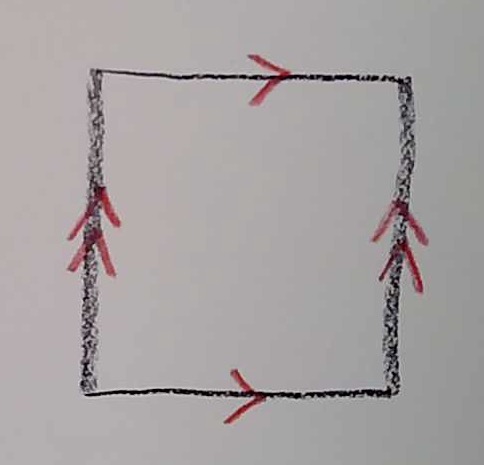
Example (a) (pages 17–18)
Note that there are infinitely many points in this sample space. However, almost all the points are represented by a finite string of T and H. That is because, by definition, we agreed to stop flipping the coin as soon as an H appears. So his E_1, E_2, E_3, etc are the only possibilities (right?).
The only infinite string is if a head (somehow) never comes up. So E_0 could be represented as TTTTT… going infinitely far.
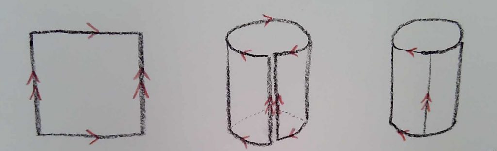
It took me a few tries to understand this example correctly. I had to re-read what the author wrote carefully. Then I imagined three actual people I know as players a, b, and c, and I talked myself through it, writing down and diagramming as I went.
“So, a and b play. Maybe a wins the first time, or maybe b. If a wins the first time, then in the second game, a plays c. If a wins, then the tournament is over. Aha, that is what ‘aa’ means! OK, now if c wins the second game…”
Exercise 19: Talk this through with yourself or a friend, and convince yourself that he has indeed listed all the possibilities of the sample space.
If you still can’t figure it out, make a note to bring it up with other students or in class.
Definition and last paragraph (page 18)
I don’t have anything to add here, but if it isn’t all clear, please make a note to ask!
6. Probabilities in Discrete Sample Spaces
OK! We were wondering before about how probabilities were assigned—in particular, if every point in the sample space had to have the same probability. Now the author is going to talk about it. Good.
If you glance ahead a little, you will see that in this chapter, he is talking about the empirical idea, and giving examples. Then in the next chapter, he is giving the formal mathematical definitions.
Personally, I find it very helpful to glance ahead and back like this as I am reading. It helps me to know what the purpose of this chapter is, and where I am in the whole voyage.
By the way, the title is again perhaps a little confusing: “discrete” means either discrete and finite, or discrete and infinite.
First three paragraphs (pages 19–20)
The author is making some philosophical remarks here.
The author’s main point seems to be to make the distinction between an idealized mathematical model and a physical scenario. No real coin flips H and T with exactly probability 1/2 each. But it is simpler to make an idealized mathematical model in which the probabilities are exactly 1/2. Then our model will apply to reality, to the extent that its assumptions are reflected in the real situation.
(And as I mentioned in the introductory lecture, even if a real coin did flip H or T with probability exactly 1/2 each, how would we ever know? We could only ever do finite sequences of flips. In a finite sequence, the number of H and T is not going to be exactly 1/2, even if the coin is exactly fair. In fact, if it was always exactly 1/2, that would be very suspicious!)
Secondarily, the author is hinting at some of the difficult philosophical problems we talked about in the introductory lecture. What does a probability of an actual event mean, anyway?
He seems to be bringing this up to say, we don’t need to answer these philosophical questions, in order to have an agreement about the mathematical axiomatic definition of a probability, which he will proceed to describe in the next chapter.
Example (a) (page 20)
If we pick balls out of a bucket one at a time, and for each ball, make a random choice of the cell to put it in, then all 27 points of the sample space in Table 1 will have the same probability, of 1/27.
Now, the “balls” may not be literal balls; they may represent any of the situations in the examples on pages 10–11, among other things. So equal probabilities may or may not be a good model.
Exercise 20: Look at the examples (b,1)–(b,16) on pages 10–11, and try to decide which ones make sense to assign equal probabilities to all points in the sample space on Table 1. (In particular, the author suggests that this does not make sense for (b,1), (b,7), or (b,11); can you see why?)
Example (b) (pages 20–21)
Note that if we don’t distinguish the balls—if they all look the same—then we could paint them red, green, and blue, and it wouldn’t change the experiment. So if we randomly select a cell for each ball as described above, then the probabilities for Table 1 are all equal, which means the probabilities for Table 2 are not equal.
Exercise 21: Under the above assumptions, find the probabilities of each of the possibilities in Table 2. (The author gives the answer on p.20; work it out yourself and then check against his answer.)
However, if the assumptions are different, then the probabilities could be different.
Amazingly, there is a physical situation where all the points of the sample space in Table 2 have equal probabilities. This is the “Bose-Einstein” statistics the author mentions, which applies to identical spin-zero particles, like photons. This makes photons more likely to “clump together” than if they were randomly distributed in the most intuitively sensible way. This is called a “Bose-Einstein condensate”.
Neither the author nor I is expecting you to understand that statement! He is just making the point that the probabilities may be assigned in a non-obvious way, (and making the connection to physics for those who have studied it, or will study it).
Example (c) (pages 21–22)
As I said in the introductory lecture, the number of heads in 100 coin tosses is not going to be always 50—it would be suspicious if it were! But it should average to 50, presumably. And it shouldn’t vary from 50 “too far”, at least not “too often”. How much is “too far” and “too often”? That’s what we want to answer soon!
Looking over it, this is another chapter with formal definitions (and even a Theorem).
As before, you should do two things:
(i) Be sure to make a note of each concept (even just listing the names, so you remember what you need to remember); and
(ii) For every abstract definition or theorem, come up with an example (which you could choose from your running pet examples, and/or the examples in the book).
I will collect all my suggestions, for examples you should be making, in the following exercise. But hopefully you are getting into the habit of doing this automatically by now!
Exercise 22: a) For the “fundamental convention”, give an example in which the probabilities aren’t all equal. (For my example, I took the experiment as “rolling two dice and taking the sum”. The sample space then consists of the numbers 2, 3, 4, …, 12. I worked out the probabilities of each of these numbers, and checked that they added to 1. You can do that one if you like, or you can pick your own.) b) Can you think of an example where there is a point in a sample space whose probability should be zero? (There was at least one example in the earlier sections.) c) Think of an example where we have already used the Definition on page 22: where we had an event A which is compound, and found its probability P{A} by adding the probabilities of all the sample points in A. (Or make up a new example.) d) In equation (7.3) on page 22, the author says that $$P(A_1\cup A_2)\leq P(A_1)+P(A_2).$$ (i) Come up with an example where the left side is strictly less than the right side; (ii) come up with an example where the two sides are equal. e) Use a few examples to check that the Theorem on the bottom of page 22 does in fact give the correct probability of $A_1\cup A_2$. f) Work through the example on page 23.
Conclusion
Whew, we’re done! Finally!
Before you go on to the exercises, take a moment now to do one more thing. Having reached the end of the chapter, you should go back and make a summary for yourself.
A good summary should be very short. It can just be a list of the sections in the chapter, and a list of what topics or important facts were in them; or you can organize it your own way. (I never feel I really understand something until I reorganize it in a way that makes most sense to me.)
OK, now you’re really done reading the chapter! Congratulations! Pat yourself on the back. Get a snack. Take a breather before you dive into the next thing, which is the Chapter I assignment!
The main structure of this class will be working through the text. However, I want to start off with some problems/puzzles/thoughts to get you thinking. I suggest that you spend some time thinking about these: it will be fun, and will help you make the material your own. I am not expecting that you will be able to find complete answers at this time, though.
I’m not asking you to hand in your work on these problems. However, if you have work on them you would like to show me, please do so! You can upload anything you want to show me to the Google Drive folder, and we can talk about it on Slack.
I encourage you to chat with other people in the class about these problems, either in person (if possible), or on Slack. However, please DO NOT look these problems up on the internet or in books. That takes the fun out of it! It’s not the point right now; I want to get you thinking on your own. And if you already know the answers, please don’t spoil the fun for others.
A lottery
Puzzle 1: Suppose that we play a lottery repeatedly. Each time we play, there is a one in one million chance we win. Suppose that we play one million times. What is the chance we win at least once?
I’m assuming here that the chance doesn’t change from one play to the next. So for example, this is not like a raffle, where there is a limited number of tickets. Every time we play, it starts fresh, and it is the same 1/1,000,000 chance to win.
Coin tosses
Puzzle 2: Suppose that I flip two coins. I show you one, and it is heads. What is the probability that the other coin is heads?
Don’t be too hasty answering here!!
Sometimes this puzzle is asked in a different form:
Puzzle 2′: Suppose that you are doing a census (going to people’s houses asking information on the people who live there). The adult who answers the door says they have two children, and one is a boy. What is the probability that the other is a boy?
Again, don’t be too hasty!
(In Puzzle 2′, we are making the (unrealistic) assumption that boys and girls are equally likely, that children are unambiguously either boys or girls, and that the assumptions of their gender don’t change. Old-fashioned assumptions! For that reason I like the coin version better, but both are worth thinking about.)
Runs
Puzzle 3: Suppose that we flip a coin 10 times, and it comes up heads every time. What is the probability that it will come up heads on the 11th time?
Note that this puzzle is very dependent on underlying assumptions, and on the exact wording. (Neither of which I have been careful about in stating the puzzle!) If you believe you have an answer, try to state the assumptions and the puzzle more carefully so that your answer is definitely true. Also, change the assumptions or the wording just a bit so that a different answer is true.
This is related to another question about runs:
Puzzle 3′: We flip a coin 10 times. Which outcome is more likely,
HHHHHHHHHH, or
HHTTTHHTHT ?
(If one is more likely, how much more likely? How about other possibilities, like HTHTHTHTHT ?)
Monty Hall
Here is a famous problem you may have seen before. If you have, please don’t give it away to those who haven’t!
Monty Hall was the host of a television game show called Let’s Make a Deal, which ran in the US and Canada through the 1960’s and 1970’s. The “Monty Hall problem” is a probability question about one of the main games in the show:
Puzzle 4: Monty Hall shows you three closed doors. He says that behind one, and only one of the doors, there is a fabulous prize; behind the other two doors are worthless joke prizes. You pick one of the three doors.
Before Monty shows you what is behind your door, he opens one of the doors you did not choose, and shows you that behind it there is a goat (one of the joke prizes).
Now he asks you, do you want to stick with the door you chose, or do you want to switch to the other remaining unopened door?
Should you switch?
What is random anyway?
What do we mean by “random”?
We might say that a coin flip is random. It comes up heads half the time, and tails half the time, unpredictably. But what does that mean exactly?
I don’t have a puzzle here, but I have some things to think and talk about.
Thing one
If we knew the initial position and velocity of the coin, and the effect of air resistance, and when and how it was caught, presumably we could predict which way it turns up. In what way is this random?
(When we were kids, my sister could not flip a coin, so she would hold the coin, show it to you, and then flip it over onto her arm. She could not be convinced that this was not sufficiently random.)
Thing two
A real, physical coin is not going to necessarily come up heads and tails exactly 1/2 the time each. It may be unevenly weighted or shaped, even just slightly. So what does it mean to say a coin flips with 1/2 probability of H or T each?
Also, even if a real coin did flip H or T with probability exactly 1/2 each, how would we ever know? We could only ever do finite sequences of flips. In a finite sequence, the number of H and T is not going to be exactly 1/2, even if the coin is exactly fair.
Thing three
In fact, if the proportion of heads was always exactly 1/2, that would be very suspicious! If we flipped a coin 100 times, and every time it came up 50 heads and 50 tails, that would be weird. We would expect it to vary from 50. Yet, we would expect it to average about 50; and we would expect that it wouldn’t be “too far” from 50, at least not “too often”.
What are “too far” or “too often”? How would we tell?
Thing four
Also, a randomly flipped coin will have longer strings of either H or T than most people expect.
One exercise I have done when I have taught statistics in the past is to give students the assignment of flipping a coin 100 times, and writing down the results (a string of 100 H’s and T’s). But there is a catch: I tell students they can choose to do the assignment honestly, or they can cheat, and just write down a random string of 100 H’s and T’s.
After they hand in the assignment, the next day I hand it back, and tell them who was honest and who cheated. This is possible because people have a very bad natural intuition of what “random” is.
Here’s another example: which of these two images are randomly generated?
From Steven Pinker, The Better Angels of our Nature
Since you know I am trying to trick you, you probably guessed it: the pattern on the left was truly generated randomly. The pattern on the right deviates from randomness, because the dots are “avoiding” each other: each new dot is less likely to land in a spot near another dot; the probability is not uniform. Our human intuition thinks of the picture on the right as “random”, but it isn’t.
Actually, the dots on the right really are avoiding each other: the image on the right is a map of the locations of glowworms on the ceiling of the Waitomo cave in New Zealand.
Here‘s a computer simulation, with which you can generate more examples of truly random dots versus “random-looking” dots.
you might initially conclude that these are random. Using the method I used to generate these, I could provide a longer sequence to a computer, and it would pass any test I know of for randomness. But if you find out that these are the decimal digits of $\pi$, starting at the 26th digit, then they are not random at all—they are totally deterministic!
So, how could you generate “truly” random digits? It can’t be done with a deterministic computer! And how would you test if a given random number generator, or physical process, was “truly” random?
This philosophical question has very practical consequences. For example, most computer security algorithms use random numbers in an essential way. But computer-generated “random” numbers are never “truly” random. Many hacks of security have been devised to try to exploit hidden regularities in these “random” choices.
You can also use the human difficulty at making random choices against them in games. For example, “rock, paper, scissors” has no winning strategy. If you choose completely randomly, it is impossible for me to choose a strategy where I will win in the long term. The best I can do is tie with you, on average.
However, most people CANNOT choose truly randomly! Therefore, a clever player—or a clever computer—can exploit hidden regularities in human choice, and they can win more than 50% of the time on average.
Try playing against the computer at this link, from the New York Times archive. (You may have to download Adobe Flash, and allow it to run on for that site.) Play it on “Veteran” mode: I think you’ll be surprised how often it is able to win! (If you have trouble running it, there are other programs that play rock paper scissors readily available; I picked this one because it beat me the worst. The other ones I found were not as impressive.)
Conclusion
These puzzles don’t touch on everything that we will be learning about in this class. But thinking about them is a good place to start!
Next time, we will start on reading the text, Chapter I, and laying some of the foundations.
You can find a pdf version of this syllabus here. You can find a more general statement of my teaching principles here.
MAT 4287 FALL 2020
Instructor. Andrew McIntyre. Email: amcintyre, then the “at” symbol, then bennington.edu. I am not physically in my office this term. The preferred way to contact me is through the Bennington Math Slack (I will send you a link to sign up); you can also contact me by email.
Me
Credits. 4 credits.
Class times and location. Tuesdays and Fridays, 8:30am–12:10pm. The course meets in the first 7 week block of the term. The first class is Friday, September 4, 2020, and the last class is Tuesday, October 15, 2020.
The class is conducted remotely and mostly synchronously (see below for details). There is an element of group work in the class; there will be some classroom space available during class hours for student groups who want to meet in person (masked and socially distanced) and who are capable of and feel safe doing so. The classroom space is in Dickinson 117, 209, 212, and 148. I will explain how to reserve these spaces for your groups after the first class.
Office hours. I will not set particular office hours this term. You can contact me any time, through Slack or email. During the term, I’ll aim to always reply within 24 hours. I can either answer questions over Slack/email, or we can set up a Zoom meeting if you prefer.
Texts. The required text is
William Feller, An Introduction to Probability Theory and Its Applications, Vol. 1, 3rd Edition, corrected printing, Wiley, 1970, ISBN 978-0471257080
The book is very expensive new, for which I apologize. It is a classic of the subject, and I did not find any good substitute. We will be working from the book quite intensively. I will be making the chapters we are working on available as pdfs, so you do not need to purchase the book. I’m sorry for that, it’s nicer to have a physical book. (In particular, the book is a good reference for many topics we won’t have time to get to.) You can sometimes find used copies of this book at more reasonable prices (try Abebooks or Alibris). However, be sure to get the 3d corrected edition; the other editions are quite different.
An alternate reference text for this class is
Charles M. Grinstead and J. Laurie Snell, Introduction to Probability, 2nd Revised Edition, American Mathematical Society 2012, ISBN 978-0821894149
This book is open-source; you can find a free pdf here. This text is not required. I am including this book because it can sometimes be helpful to have an alternate explanation for topics.
Calculators and computers. A simple scientific calculator or calculator app will be sufficient for almost all the work in this class. You will not need a graphing calculator, though you are welcome to use one if that is what you already have and you are comfortable with it. I will occasionally ask you to graph something on a computer; I recommend the free web app https://www.desmos.com/calculator.
What this class covers. This first course in probability will take a classical approach, following the classic text by Will Feller, An Introduction to Probability Theory and its Applications. In particular, the topics will include: sample spaces, conditional probabilities, independence, random variables, expectation and variance; the binomial, Poisson, and normal distributions; the law of large numbers and the central limit theorem; random walks; and Markov chains. The course will not cover measure theory or formal proofs, but there will be proofs at an appropriate level of rigor. The aim will be to get a deep understanding of the classical concepts, mostly in the discrete case. Students should be well set up to learn more on continuous distributions and Bayesian approaches in future courses if needed. The class should be of interest for both theoretical and applied purposes. The class will be a prerequisite for Machine Learning in Spring 2021.
Prerequisites. Some familiarity with the language of set theory, the binomial theorem, exponential and log functions, and infinite series will be helpful. If students have taken MAT 2410 Logic, Proofs, Algebra, and Set Theory and MAT 4133 Calculus A, they will be well-prepared, but students need not have taken those particular courses. I will make available “preamble assignments”, which students can work on before the class begins to develop the necessary skills.
Work expected. In this class, I am putting an emphasis on reading and understanding the text. I will ask you to read the text, make notes, comments, and your own examples, and contribute to class discussion boards on the text and problems. You will do collaborative work on problems, and assignments that you will hand in. I also encourage you to spend time helping your classmates understand the material, and will explicitly credit you for that work as well.
The usual expected workload for a 4 credit class is 10 hours per week, meaning 4 hours per week in class and 6 hours outside of class. (The logic of this is that a full 16 credit schedule would then be 40 hours per week of work.) Because this class is 4 credits in 7 weeks, the expected workload is 20 hours per week, meaning 8 hours of designated class time, and 12 hours spent on work outside of class time.
You may not be spending fully 20 hours every week, but if you spend much less than that, it will be difficult to get full value from the class and to do well. On the other hand, I am not expecting more than 20 hours per week. If the class finds that the average student time is getting close to or above that number, then I will adjust the expectations to keep it under 20 hours for most people.
I recommend scheduling 20 hours per week, (including class time), and doing the best you can with the work in those 20 hours. If you do this, you will be successful in the class, even if you don’t complete all problems.
I understand that life may interfere with regular commitment to the work, particularly this term. If you are having difficulty putting in the time, please let me know as soon as possible. I will do my best to be flexible and help you stay on track. I am committed to making success in this class possible for any student who can put in the time.
How to submit work. I will make a Google Drive folder for you to upload your work. I will expect you to upload your work on assignments. If you worked on problems but can’t solve them, submit what you do have: partial solutions, strategies, ideas, or just a sentence trying to explain why you are stuck.
I encourage you to also upload notes and other evidence of your work. In ad- dition, each week I would like you to write a short list of what you have been spending time on that week: reading the book, working with others, explaining things to others, and so on.
One way of doing this is I would recommend is to keep one bound notebook, in chronological “journal” format. Label each item (“assignment”, “lecture notes”, and so on), but just write in the order you are doing the work. Talk to yourself in this book—that helps a lot with your thinking, and it helps me to see what you are thinking. (e. g. “I spent two hours reading Chapter I, and made the notes above. The main thing I don’t understand is. . . ”). Then, you can just upload new pages of your journal/notebook as you complete them.
However, you don’t have to do it that way; any method that allows you to stay organized, and allows me to see what work you are doing, is fine.
I am not focused on specific due dates. I will make recommended due dates for assignments, but each week what I want to see is the work that you have completed that week. If you don’t get an assignment completed one week, you can continue submitting that work in following weeks until you have completed it. (Though it may sometimes be better to leave an assignment aside and concentrate on newer work; I’ll make suggestions to you about that, see the following.)
A technical note: please get a scanning app for your phone that will allow you submit your work as pdfs. There are a number of free apps available. These apps have a number of algorithms that make the scanned material much more legible than simply taking a photo. Also, they allow you to scan work as multiple-page pdfs, which is much easier for me to read than having a list of single pages in the folder.
Please put the date of your submission in the file name; in fact, just using the date as the file name is often the easiest way for me to navigate your work. For example, a filename like “2020-09-07-2” for the second thing you uploaded on September 7 keeps things in clear order. However, you are welcome to organize your folder however you like, as long as it is easy for me to navigate and find your work.
Feedback and assessment. Each week, I will look over the work you have uploaded to the Google Drive folder. I will let you know the day I am doing this once we get the term started. After looking over your work, I will write a narrative comment, and send it to you by Slack.
Many of the problems have final answers given, or can be checked by consistency or other means. So I will be focusing less on checking answers, and more on more global issues. For example, I might make comments like “you need to show more of your reasoning on more problems”, or “there are some numerical errors in the early questions, please check those again”.
I am also asking you to write something at least once a week about how you are spending your time; for example, you might be spending a lot of time on reading, or working with others, that isn’t evident in your written work.
I will also try to make suggestions about how you are spending your time, and about what will help you as you proceed. For example, I might make comments like “you don’t need to write quite so much”, or “you can skip some questions on this last assignment and concentrate on the current assignment”, or “try to go back and clarify these particular concepts in the previous chapter, they are holding you back now”.
You are welcome and encouraged to write back and make this a dialogue, about how you are doing, what is going well, and what you need to work on.
Evaluation. There will be a “midterm” evaluation (in roughly the fourth week), and a final evaluation. For both evaluations, I will write a narrative paragraph, and I will ask you to write a self-evaluation narrative paragraph. If you are requesting a grade, I will ask you to propose a grade and I will assign one, for both midterm and final.
The criteria I use for your evaluation will be the same that I ask you to use for your self-evaluation. It will include:
whether you are spending sufficient time and attention on this class • how thoroughly you are reading and understanding the text
how thoroughly and correctly you are solving the problems
how persistent you are with difficult problems
how creative you are with challenging problems
how clearly and carefully you are writing your reasoning
how much of the work you are completing
how well you are contributing to collaborative work
how well you are contributing to class discussions (in whatever form)
how well you are helping other students in the class, if applicable
how consistent your presence in the class is (see below)
The most important criterion is the time and effort that you are putting into the class.
I expect that, in most cases, your self-evaluation and my evaluation will be in general agreement. If we disagree, we will compare records; I may ask you to show me work on problems, or answer questions about concepts, if we disagree on how completely you have solved or understood something.
I will be responsible for the final narrative evaluation and grade that goes on your transcript, but in all but exceptional cases we should have reached consensus by then.
Note that it is never too late to “make things up”; if you figure out problems or concepts several weeks later than we covered them, you can always submit work to the folder to show me your progress. I will only “count” how solid your understanding and work are in the end, not when you got there or how long it took. (That said, since this is a seven week class, be aware that you won’t have much time to catch up if you get too far behind!)
Notebooks. It is very important to keep a clear and organized notebook (or equivalent system) for this class. You will need records of your work to be able to show me, and you will also need a clear way to refer to and build upon your own work.
I recommend keeping a bound notebook (like a composition notebook), for this class only. Write your thinking about the problems in a journal format. Also write class notes, solutions to problems, and summaries. This will help keep your thinking in one place. Number the pages, and put a table of contents at the end.
You may prefer to have a different system: perhaps you could have a bound notebook for notes and journal work, and write problem sets up separately. Or you could use a looseleaf binder, or a system of folders. Whatever you choose, your work should be accessible, clearly written, and understandable to both me and you. Don’t assume that you will remember what you were doing later—write your explanations down in full as well as your computations.
Note that, since the work will be submitted by scans, if you like, you can have your problem set solutions in the same bound notebook that you use for notes and thinking.
A note on collaboration. For much of this class, I will be expecting you to work with other students. This might seem like it would be unproductive, if neither of you know what is going on—“the blind leading the blind”. But in fact it can be very useful to talk through your thinking with another person. You say what you are thinking, explain where you are stuck, the other person does the same; and in articulating your thinking and difficulties aloud, it becomes clearer where to go next to resolve the problems.
This is not unlike how research mathematicians work together. We don’t have a teacher who knows the answer; perhaps no-one does. We throw out ideas, and then try to test them: e. g. “if that was true, then how would it work in this simple example?”. We try to generate more examples to test ideas, and if we think we have a solution, we try to verify it from different directions.
A large amount of class time will be devoted to collaborative work. I would also encourage you to work with other students outside of class. This is particularly helpful when you are having trouble persisting with problems when you are stuck— having someone else there can really help you push through.
For this class, I want to go one step further: I want everyone to succeed together. I want to explicitly encourage you to help each other. It’s not a good idea just to tell someone how to do a problem, because then they don’t really learn much. But you can give hints, make suggestions, talk things through together, and try to explain concepts in different ways. If you are spending time helping other students, please let me know; I will explicitly include this in your evaluations.
All that said, it is also important to be able to do work on your own, and to be sure that you truly understand things yourself and are not merely following along. Here is a good rule of thumb: collaborate with other students verbally, and on whiteboards. But when it comes to write down the solution, do this on your own, without referring to what you wrote collectively. Write the solution from your own thinking, do not just copy.
A note on lecturing. A major emphasis in this class is to help you learn to read a mathematics text yourself, as much as possible. This will make you more able to learn more probability (and more math) independently in future, beyond the confines of this class.
For this reason, I will be avoiding lecturing on things which are contained in the text.
I will make written “lectures”, which will often be largely reading guides for the text. I may give you examples or a short overview to start with. Then I will give section-by-section suggestions (particularly for the early chapters) about how to read the text, and how to figure out the difficult points.
We will not spend the entire 4 hour scheduled meeting time in class together. I will be available on Zoom for the full 4 hour meeting time, but not in formal lecture. Typically I will expect something like this: we devote an hour or so to collaborative work and reading (with me available for questions), then an hour formal “lecture” (which will be mostly me addressing problems or tricky points which many people encountered, plus class discussion), then an hour of you working on problems in groups and me answering questions, with some breaks in between.
My view is that the class should primarily offer things that you could not get by simply working on your own. There are two elements to this: one is collaboration with others (see the note above). The other is feedback as you are working. I will get you to start on problems on your own. If you reach a point where you are stuck, I will use my experience to try to give the best possible hint or suggestion appropriate to the point you are stuck at. As much as possible, I will try to only make suggestions that you could have thought of yourself. In this way I hope to help you improve your ability to figure out this sort of material on your own.
Presence policy (including attendance). It will be important to have a consistent presence in this class. Particularly on the shortened schedule, if you are not present for even a short while, it will be difficult to catch up.
I understand, however, that there could be many issues which might sometimes make it difficult or impossible to attend our scheduled class sessions. Therefore, instead of an “attendance” policy, I am making a more broad “presence” policy. It is required that you maintain a consistent presence in this class through all 7 weeks. Not having a presence for one week or more (total) is grounds for concern, and could possibly affect your evaluation.
Presence includes
attendance at scheduled classes
contributing to class discussions, either during scheduled class time, or on Perusall or Slack
participation in collaborative group work, either during scheduled class time or outside of it
helping other students, either during scheduled class time, or through Slack
contacting me with questions, or discussing problems and ideas with me I do not expect that everyone is doing all of these things all the time. But you can make up for one with the other; for example, if you cannot make it to a scheduled class, be sure to find time to work with students in your group, to talk to me, and/or to participate in online discussions. I should be able to see evidence of your presence consistently every week. If I don’t, I will bring that up in the weekly feedback.
Weekly schedule.
Class
Date
Chapters and Topic
1
Sep 4
I Sample Spaces
2
Sep 8
3
Sep 11
V Conditional Probability and Independence
4
Sep 15
5
Sep 18
VI Binomial and Poisson Distributions
6
Sep 22
7
Sep 25
VII and X Normal Distribution and Central Limit Theorem
8
Sep 29
IX Random Variables, Expectation, Variance
9
Oct 2
10
Oct 6
III and XIV Fluctuations in Coin Tossing and Random Walks
11
Oct 9
12
Oct 13
XV Markov Chains
Classroom Inclusivity. Everyone is welcome in this classroom, and in mathematics. Please be kind and respectful to one another.
IF YOU ARE NERVOUS ABOUT BEING IN THIS CLASS, please know that, in my experience, everyone can do mathematics, and do it well. You may have had negative experiences with math, and you may have had assumptions made on your ability for invalid reasons. It’s normal to be nervous. You can do this, and you will be supported here.
IF YOU FEEL CONFIDENT ABOUT BEING IN THIS CLASS, (you might belong to both categories!), please be kind and respectful to your classmates. Do not talk over them, or make it seem like they should know things that they don’t. You will find, as the class goes on, that we are all struggling with math problems in our own way. We are all in this together.
IF YOU ARE MADE UNCOMFORTABLE IN THIS CLASS for any reason, please talk to me about it. (Aside from being uncomfortable about hard problems, but you can talk to me about that too!) I will do what I can to solve the issue. If I do not resolve the issue, or if I am the one making you uncomfortable, please talk to a college administrator (e. g., from The Office of Diversity & Inclusion, Student Life, or Academic Services) or other faculty member.
Here’s the official statement: Bennington College is committed to fostering the intellectual growth of all students, and to creating a learning environment where human cultural diversity is valued and respected. To that end, in this course all students can expect a respectful, welcoming and inclusive environment. I hope that all students in this course will openly share their unique perspectives and, just as importantly, respect the perspectives, comments, and contributions made by every other student and guest that participates in this course during the term. If you feel that at any time that this goal is not being met, please don’t hesitate to see me, or speak with a college administrator (e. g., from The Office of Diversity & Inclusion, Student Life, or Academic Services) to share your concern.
Academic Accommodations and Health Resources. I am happy to work with you on any needed accommodations. Please let me know the situation.
Here is the official statement: Bennington College provides reasonable accommodations to students with documented disabilities when such accommodations are requested and necessary to ensure equal access to College programs and facilities. If you believe you are entitled to an accommodation speak with Katy Evans, the Academic Services and Accommodations Advisor, about any disability-related needs. If approved, you will receive a memo detailing your specific accommodations; it is your responsibility to provide me with the memo and discuss the implementation of accommodations. Note that I will not be aware of your needs if you do not share this memo with me. Accommodations are not retroactive, so the sooner we meet to discuss your needs, the better. Also, students experiencing mental and/or physical health challenges that are significantly impacting their academic work are encouraged to speak with their faculty advisor and member of Academic Services (academicservices@bennington.edu or 440-4400) about the impact and to connect with resources through health and psychological services (440-4426 or 440-4451).
Statement on Basic Needs. At Bennington College, we understand that basic needs (food, housing, and wellness) have a direct impact on academic performance, mental-emotional-physical health, professional development, and holistic success of our students. If you have a personal circumstance or need that will affect your learning or performance in this course, please let me or your faculty advisor know so that we can direct you to available resources to help support you during the term.
Conclusion. You can find a more general statement of my teaching principles here. Please contact me if you have any questions at all!
“Immaculate Heart College Art Department Rules”, by Sister Corita Kent
Hi! Welcome to Probability Fall 2020!
I probably could have brushed my hair for this. But I’m trying to keep this informal!
In this post, I want to cover the usual “first day of class” topics. I’ll talk about the setup of the class. I’ll outline the topics and goals. All of this is covered more formally in the syllabus, which you should read at some point. Here, I’ll talk about the structure of the class more informally.
There are some parts of the class I want to decide about collectively with all of you; I’ll talk about that at the end.
To start with, welcome back to Bennington! (In person or virtually!) This has been a very strange situation, and I’m sure many of you have had a very stressful and/or weird spring and summer. I want to acknowledge that, and build it in to my teaching this term—more on that at the end.
I’m glad to be back! It was difficult to suddenly switch to remote learning in the Spring, part way through the term. I’m hoping that remote/hybrid learning will work better now that I have had some time to plan and prepare.
I’m optimistic for this class, and excited to be teaching probability! It’s probably the standard math topic I know least well, and I’ve never taught it before. It’s an interesting subject, and I’m looking forward to getting started!
Organization of the class
My idea for the organization of the class is to have five main elements:
Written lectures, in a “blog” format (like this one). These will be informal and conversational. A lot of what I will be doing is giving you a guide to reading the text. I will ask questions in these lectures, which I want you to try to answer. I will not be collecting your work on these questions. You should aim to read the written lecture, and at least try all the problems, before the class time, if you can.
Synchronous video lectures. These will happen during the scheduled course time, but they won’t take up the whole time. Probably they will be about two or three hours per week total. These will support the written lectures. The video lectures may have more explanation, but they will not add anything new. In the video lectures, I will answer questions about the written lectures and the reading. The video lectures will also be recorded so you can watch them later. After the video lecture and class, you will probably find it necessary to go back and work through the written lecture a second time (at least).
Synchronous individual and group meetings and work. Most of the scheduled course time, I will not be lecturing; you will be working, either individually or in groups, and/or I will be meeting with you, either individually or in groups. We will work together to figure out the most efficient use of class time, to help you work through the material. I’m thinking that we will start each class meeting with an hour of you doing reading and work, and with me available on Zoom; a break; then an hour of more formal lecture/class discussion; another break; then another hour of you working and me available again.
Asynchronous discussion and meetings. It can be difficult to have a good class discussion on Zoom. I am hoping that Slack will be a replacement for that. In the #probability channels, you can post questions to the whole class and me, as well as thoughts about the material, interesting links, etc. You can also send me individual direct messages with questions, which only I will see. I am planning to do a lot of answering questions, and feedback on assignments, through Slack. I can also switch from text to video on Slack, if you want to discuss something that is difficult to do over text.
Formal assignments. Once you have worked through the written lecture, and have done the problems there, you should work on the problems on the formal assignment. I will ask you to write up these answers fairly carefully. They should be written up clearly enough that someone who did not know the problem would be able to learn how to do it from your solution. I will have you submit your solutions to the assignments on a Google Drive folder, which will be shared between you and me only.
The text
The main element of this class is the textbook,
William Feller, An Introduction to Probability Theory and its Applications, third edition, corrected printing, John Wiley & Sons 1970.
I apologize for the very high price of this book. Here is a link to a pdf. Print is nicer, of course; you can sometimes find reasonably priced used copies of this book. Try AbeBooks or alibris. (Be sure to get the corrected third edition; the other editions are quite different.)
Why did I choose such an old and expensive book? This book is a classic, and rightly so. It was the first comprehensive introduction to the subject in English, written by one of the masters of the subject. I spent a long time looking at all the probability books I could find, and none of them was as clear, as deep, or as interesting as this one.
The book is slightly old-fashioned in certain respects. In particular, there are two newer topics, that go by the names of “maximum likelihood” and “Bayesian probability”, that are not much covered in the book and are popular now (partly due to an increase in available computing power). My logic was that it would be better to get a solid grounding in the classical theory first, which this book provides. If you have that, the newer topics will not be difficult to pick up as you need them.
Also in that respect, I am sticking to problems that are done by pencil and paper, or at most a calculator. Some modern books do a lot of computer simulations. I am intentionally NOT doing that in this class. I think the computer approach makes sense, and has some definite advantages. However, overall, I think it is better to have a solid conceptual understanding first, and then to go to computer simulations later as needed.
(If you would like an alternate reference book, I would recommend the free book by Grinstead and Snell. It is pretty good, more modern, and close in structure to our class. Sometimes it can be helpful just to see an explanation in different words. It also describes a number of computer simulations which you can try out if you are interested.)
Specific goals of the class
I am planning this class as a classical, thorough introduction to the concepts of probability. The specific topics I’m planning are:
Chapter I: Sample Spaces
Chapter V: Conditional Probability and Independence
Chapter VI: The Binomial and Poisson Distributions
Chapter VII and X: The Normal Distribution and the Central Limit Theorem
Chapter IX: Random Variables and Expectation
Chapter III and XIV: Fluctuations in Coin Tossing and Random Walks
Chapter XV: Markov Chains
Of course, these titles won’t make much sense until we get to them! For now, I would just say that these are standard, foundational topics, and that they should leave you well-prepared for using probability theory in future (including for the Machine Learning class in Spring, if you are planning to take that).
Note that the book contains a LOT more material than we will be able to cover. Part of my intention of assigning this book was so you could get used to it; then, if you want to learn about any of the many other topics covered in the book, you will already be familiar with the style and structure.
In each lecture and assignment, I will try to identify the main concepts and skills that I am trying to get you comfortable with.
More general goals
Because the textbook is so good, I want to use it a lot in this class. On a more general level, I am hoping that this class will help you build up or improve your skill at reading this sort of mathematical text. That way, when you need to learn more probability (or other math) in future, you will have an easier time doing so independently.
To that end, I am NOT going to explain all topics in the lectures. Instead, the lectures will be a guide to reading the text. I will try to prepare you for the reading, and I will try to provide additional explanation where needed; but I will try NOT to straightforwardly repeat what is already said in the text.
Also, this subject will provide interesting applications to things you may have seen in a more theoretical form in Logic and Proofs or Calculus (if you took those classes). Overall, I hope that you will leave this class with improved general mathematical skills, conceptual flexibility, and confidence!
Why I’m not going to cover current topics
Trigger warning (for this section only): illness, racism, other stressful topics…
Originally, when I was first planning this course earlier in the summer, I was thinking of MANY applications of this material to current events. There are natural connections of the probability theory we are learning to the coronavirus pandemic (testing, false positives and negatives, predicting true rates from testing rates…), to racism (inequality and police violence, analyzing other structural inequalities…), to politics (voter suppression, gerrymandering,…).
This seemed like a good opportunity, and I was planning many examples.
Then I did some reading on trauma and education, by people who have thought about this stuff a lot and have done a lot of research, and it changed my mind.
For some of us—for some of you—these issues are, or are going to be, not just abstract, but painfully personal. This would be true any time, and is particularly true this year. Maybe a family member is sick, or imprisoned, or something worse. If that is the case for you, then seeing examples like this in class is going to remind you of your trauma or stress, just at the moment when you are trying to forget it and concentrate on your work. If you have a lot going on, probably it is going to be hard to stay focused on your work anyway; I don’t want to make it harder.
I’ve given this a lot of thought, and I think that, while it would be interesting to cover current topics such as these, the potential for harm is just too great.
For that reason, I promise to keep all the examples neutral: cards and dice and such. When there is a somewhat current topic, I’ll keep it as neutral as possible. (For example, false positives and false negatives for disease tests is a standard probability example; I’ll keep it as nondescript as possible.)
I’ll set things up so that, if you are interested, it should be clear how to apply the ideas to current topics (and you can think of doing so as an optional exercise!). If you would like to talk about examples relevant to current topics, I’m happy to discuss them with you privately (you can direct message me in Slack).
Like with the computer stuff, I will try to provide you with the foundations, so that if you want to go on to apply these ideas yourself, you have all the tools to do so.
The workload for this class will be 20 hours per week, including the 8 hours of scheduled synchronous time.
I will probably end up assigning more work than is really feasible to do in this time limit. That is OK. If you are spending 20 hours per week, that is both sufficient and necessary to do well in the class. You should submit whatever work you have, including partial answers or ideas (more on that below).
Rather than thinking about a to-do list of readings and assignments, I would recommend just blocking out 20 hours per week in your schedule. This could be 4 hours each weekday (including our class times on Tuesdays and Fridays), with weekends off, or you could arrange it differently. During that time, do as much as you can on the work for this class.
It does need to be 20 actual hours, not half-attention shared with internet browsing and so on. This is really tough: it’s a lot of time to concentrate on math, and it takes practice. If you can’t keep it up in one session, don’t worry, just resolve to keep your time block tomorrow.
Keeping a record of your work
I recommend keeping your work in a journal format. Get a bound notebook (like a composition book). Write all your work in there, in chronological order: notes on classes, notes to yourself, work on exercises and assignments, examples you are making up.
Lynda Barry, Syllabus (published as a composition book!)
The notes to yourself are particularly important. This will help you in your thinking, and it will help me to see what you are thinking. You can write things like “I am confused about this question; how is it different from xxx?”, or “I think I need to apply the binomial theorem, but I’m not sure which variable is which”, and so on.
Here’s an example of journal-style notebook keeping. These examples are from Dan Quillen, a mathematician; you can see them here. You’re not going to understand the content, but I want to point out the style. Every page is numbered—I find this really helps with organization, even if you don’t use the page numbers much. The notebook starts with a table of contents:
Here is a sample page. Don’t worry about the content. Note that the style is of talking to oneself. Note in particular: “What I am looking at is…”, and “The problem I am having is…”
You don’t HAVE to keep your notes this way. You can organize them differently if you like, whatever makes the most sense to you. However you do it, you should make sure that it is easy for both you and me to see what you’ve done, to understand what you’ve done (even later after you’ve forgotten the set-up), and to find what you’ve done.
How to submit work
I will be creating a Google Drive folder for each of you. This folder will be shared between you and me only. All your work will be submitted in this folder.
Please use a pdf scanning app on your phone. There are several free ones available. This will align and filter the work to make it more legible, and it will create multiple-page pdfs. It can be quite difficult to read your work in photos, which are often upside-down or misaligned, in varying resolution, and only come one page at a time.
I recommend just updating the work you have on a regular schedule, whether or not assignments and other work are completed. The “journal” format of keeping notes and work functions well with this: just keep updating new pages of your journal/notebook as you have them.
If it isn’t obvious from your notes and work, you should make a note of time you spent, so that I know about it. For example, if you spent a long time reading the text, but don’t have notes on it you want to upload, or if you spent a long time explaining material to another student, these are things that are helpful for me to know. If you are keeping a journal format, you can just write those as “diary” entries: e.g. “Tuesday Sep 8, spent 2 hours working with group, mostly on beginning Chapter I questions, not much written down but understand the questions better now”—that kind of thing.
It’s more important for me to see your steady progress on the work, than to see completed assignments as full units. (Though you should aim to complete the assignments if possible!) I will have suggested due dates for exercises and assignments, but if you don’t get something done one week, you can submit it the next.
Once a week, I will be looking at the work you have uploaded, checking it, and giving you feedback.
The feedback will mostly be a narrative paragraph, which I will send you on Slack (visible only to you).
Many of the questions either have the final answers given, or can be cross-checked in various ways, so for the most part you will be able to check whether your work is correct. I will check some for correctness, but mostly I will be looking at bigger issues. For example:
Do you need to be writing more detail in your solutions, at least some of them? If you just have some numbers without explanation, I may not be able to see your reasoning and tell if you are understanding.
On the other hand, maybe you are writing too much for every question, and having trouble getting through everything; if that seems to be the case, I will let you know that you can be more brief.
If you are getting stuck on particular things, I can make suggestions about what you need to work on more.
If you are getting hung up on a particular reading or assignment, I might suggest moving forward and then coming back as needed.
If you’re having trouble getting a sufficient amount of work done, I’ll ask you about what is causing trouble, and we can work on a solution.
I think I will be setting a particular day of the week to do this: maybe Wednesdays? I will let you know.
You are encouraged to respond to my feedback as needed, and ask follow-up questions or make additions.
Support
Please ask questions! There will be time to do so in class. You can also write me in Slack any time. You can ask particular questions about particular problems (“am I doing this right?”, “how do I get started, I’m stuck”), or more general questions.
If you are comfortable doing so, I recommend asking questions in class, or posting questions to the Slack channels, so the rest of the class can either see my responses, or provide their own responses.
I also strongly encourage you to help each other in this class. I see the success of this class as being a group project: I want ALL of us to work towards ALL of us understanding this material. There is no “curve”: helping someone else will not hurt your standing.
In particular, if you are helping others, I would like to credit you for this on evaluations. So if you have been helping others, please make a note of it in your submitted work or on Slack. And if others have been helping you, please let me know that too, so I can credit them appropriately!
(“Helping” of course doesn’t mean doing other people’s problems for them, or giving them the answers. That doesn’t truly help in the long term anyway. It means discussing, making suggestions, providing hints, and talking through the concepts.)
Please try to make space for one another. Listening is as important as speaking. We are all in this together. Please try to be supportive and kind to one another!
In conclusion
I haven’t covered the whole syllabus, so please read through that if you haven’t already. You might be also interested in my general principles for teaching math.
I’m looking forward to this class! I’ve never taught probability before. It’s going to be fun. It’s going to be tough to feel connected with this distance learning, so please talk to me, talk to your classmates, ask and answer questions.
Here are some follow-up questions to class, and to the “parable” I posted last time. (They are certainly not the only questions one could ask—I encourage you to think of more!)
In talking about this, it will help to use the term “countable”. A set is “countable” if it can be put into one-to-one correspondence with the natural numbers, {0,1,2,3,…}. In class, I showed that the even numbers are countable, and that the rational numbers (all fractions a/b, where a and b are integers, b not zero) are countable. I also showed that the real numbers in the interval [0,1] are not countable; that is, the real numbers are a “larger” infinity than the rationals or the naturals. You can take those facts for granted in what follows.
Question 1: Let’s say that god starts with a countable number of angels. (Since they are countable, god might as well give them identification numbers: 0, 1, 2, 3, …) This question is about how much room god needs for the angels. The rule for an angel is that each angel can take up as little volume as god chooses; but an angel cannot take up zero volume. (a) Explain how god can fit any finite number of angels into a finite volume. (b) Explain how god can fit ALL the angels into a finite volume. (Hint: Look back at our discussion of calculus, and Zeno’s infinite series.) (c) Now, suppose god is building clubhouses for all the angel clubs, potential or actual. The rules for a clubhouse are the same as the rules for angels: god can make them as small a volume as she likes, but she cannot make them zero volume. Explain why she cannot fit all the clubhouses into a finite volume. (Hint: This one is a little tricky. Suppose god has a finite volume V to work with, and suppose the clubhouse volumes are all chosen. List all the clubhouses of volume bigger than (1/2)V—how many can there be? Then list all the clubhouses of volume bigger than (1/3)V that you haven’t already listed—how many can there be? By continuing this way, show that the number of clubhouses that fit into the finite volume must be countable. Because of this, conclude that not all clubhouses can fit into the finite volume.
Following up on the previous question: suppose that god had infinite space to work with. Let’s take “infinite space” to mean ordinary R^3 coordinate space, all points with x, y, z coordinates, where x, y, and z can be as large as we like. Even in infinite space, the number of clubhouses that will fit are still at most countable. For this reason, the clubhouses will not all fit, even in infinite space.
Question 2 (optional): Here is the outline of the argument why the number of clubhouses in infinite space is still countable. (a) Explain why infinite space R^3 is made up of a countable number of pieces of finite volume. (You could use cubical blocks and a spiral counting argument like I did in class. More simply, you could imagine concentric spherical shells.) In each of those countably many pieces, only countably many clubhouses will fit, according to the previous question. (b) Explain why, if we take a countable collection of volumes, each containing countably many clubhouses, we still get only countably many clubhouses in general. (Hint: Since the collection of volumes is countable, we can label them with natural numbers, say V_1, V_2, V_3, … Now, within each volume, the collection of clubhouses is countable, so we can also label them with natural numbers. The clubhouses in V_1 we can label C_11, C_12, C_13, … The clubhouses in V_2 we can label C_21, C_22, C_23, …. Now, there are different ways you can show this collection of all C_ij is countable. One way is to think of each clubhouse as labeled by a pair (i,j), draw all the pairs on an x-y plane, and make a zig-zag argument like I did in class.)
The arguments above lead to a very weird thing that is difficult to imagine: let’s consider a 1 x 1 square in R^2, the ordinary x-y plane with real coordinates. In class, I proved that the rational numbers are countable. By the same argument as the last part of the previous question, the set of all points in the square with rational coordinates (x and y both rational) is also countable. Because there are infinitely many rational numbers between any two numbers, if you imagine the set of all points with rational coordinates, it would visually fill up the whole square. (Right?) Mathematically, there would be points missing, but for any missing point, there are rational points which approximate it as closely as you like (in particular, more closely than the resolution of any actual picture).
Suppose that we surround each and every rational point by a small square. And suppose that we add up the area of all those squares. How much area do we get? Any guesses?
. . . . . . . . . . … Certainly it seems like the total area should be at least 1, right? Because the squares would effectively have to cover over the entire 1 x 1 square?
No! In fact, I can find such squares with area less than 1/1000.
Here’s how: since the rational points are countable, I can label them in order: p_1, p_2, p_3, p_4, … Each p_i is a point in this square, with rational coordinates; and every point in the square with rational coordinates appears somewhere in this list.
Put a little square box around point p_1, and make the box small enough so it has area 1/2000.
Put a little square box around point p_2, whose area is 1/4000.
Put a little square box around point p_3 of area 1/8000.
God is busy setting up the universe. (If you’d prefer I not be flippant about god, please take it to be an alternate universe…)
God starts by creating angels. Since she has a potentially infinite set of tasks to perform, she creates infinitely many angels. She can do it, she’s god. And she is a “do it right the first time” kind of god: rather than create some angels now, and then realize she needs more later, she will create angels for every conceivable task. Hence the infinity of angels.
God foresees that the angels may want to form associations with each other. For example, all the angels responsible for the animals might want to form their own club; all those responsible for properties of numbers might want to form another; and so on.
Now, as I said, god does not like to do things twice. So, thinking ahead, she creates ALL possible clubs. For every possible collection of two or more angels that could exist, she enters it in a catalog, gives it a provisional name, prints up membership cards, builds a clubhouse. (She doesn’t give it a final name, because she doesn’t know what that particular collection of angels might want to form a club for. The angels do have some free will, after all.)
Being a fan of order, God decides to assign a leader to each potential club. For every potential club, there will be some angel that is its leader. Should that collection of angels choose to form a club in future, the clubhouse will already be built, and the leader will already be chosen. It will fall to the leader to collect membership dues, keep careful minutes, and fill out the necessary forms. (God likes order, as I said.) Since the duties can be somewhat onerous, god decides that each angel will lead only one potential club at the most. No angel is responsible for two or more clubs, potential or actual.
As she begins the assignments, she realizes that it will not always be possible for the leader of a club to be a member of that club!
Problem: Pick any three angels, let’s call them A, B, and C. (It wasn’t until later that angels got into fancy names.) a) List all the possible clubs that A, B, and C could potentially form. b) Explain why it is not possible that every potential club can have a leader who belongs to that club.
Well, no matter. God can start assigning leaders to some clubs who do not belong to the clubs they lead. There are infinitely many angels, after all, to assign to these infinitely many tasks. So the catalog is written, with all potential clubs of angels, and for each potential club, an angel leader, who will be called upon should that club decide to form. The leader may or may not be a member of the club that they are assigned to lead; no matter.
Time goes on, various clubs form, and leaders are called upon, referring to the infinite catalogue. All is well.
Then one day, some angels are talking on one of their AOL message boards (these were still the early days of the universe). The group who are talking consists of several angels, who each led groups to which they did not belong. They felt that it was difficult to lead a group, if you did not belong to it. The group felt that you did not understand their issues, and (the angels suspected) did not always invite you to their pizza parties.
These angels, (let us call them ostracized angels, in view of their social difficulties), decided to form a club. It would be a club for all angels who did not belong to the clubs (potential or actual) that they led: the club of ostracized angels. There would be much to discuss; no longer would they feel so left out.
Excited, the angels made a list of all angels who were ostracized in this sense. They took the list, and looked it up in god’s catalogue: recall, in god’s infinite foresight, she has provided ahead for ALL possible clubs that might form in future. Somewhere, waiting for them, was a clubhouse, all fitted out with chairs and a mediocre coffee maker.
And, most importantly, (for angels love hierarchy), they excitedly looked in god’s infinite catalog to find which angel she had chosen to the lead them.
There, they made a troubling discovery.
Problem: What was the troubling discovery? (Think about it for a bit, and then scroll down to the bottom of this page for a hint.)
Problem: What is the meaning of this disturbing outrage? What can we conclude from it?
Hints follow, don’t scroll down until you’re ready for the hint . . . . . . . . . . . . . . . Are you sure you’re ready? I think you might still be able to figure it out on your own. . . . . . . . . . . . . . . . . . Are you really sure? There’s time to turn back. . . . . . . . . . . . . . . . . . . . . . . . OK, OK, I could do this all day.
Here’s the hint: it would be terribly ironic if the leader of the ostracized angels was herself ostracized, would it not? Is she? Or isn’t she?
In this lecture, I want to talk about the Möbius strip and its cousins, the non-orientable 2D spaces. (And I want to talk about what “orientable” means.)
I’ve talked with you in class about some of these things; I want to back that up here, and to provide some more details. Then I want to go a bit further. The relevant text for this is The Shape of Space, Chapter 4.
The Möbius Strip
Let’s recall the Möbius strip. There are two different spaces I have been talking about, and I’ve been calling them both the “Möbius strip”, so let me set the record straight here.
Actually, while I’m at it, I’ve been calling two different spaces the “cylinder”, so let me come clean there as well.
On the one hand, I can start with an infinite strip in the 2D Euclidean plane, bounded by two parallel lines on its sides, and I can “glue” the left side to the right side:
The infinite 2D cylinder, intrinsically.
This can be embedded in 3D, as the surface of an infinitely long, straight, circular tube:
The infinite 2D cylinder, embedded in 3 dimensions.
I will call that one the “infinite cylinder”.
On the other hand, I could start with a rectangle, and glue together two of the sides, keeping the orientation straight:
The finite 2D cylinder, intrinsically.
This one I’ll call the “finite cylinder”. It also has a uniform locally Euclidean geometry, but it is finite in extent, and it has a boundary, consisting of the top and bottom edges. A 2D inhabitant of this universe can “fall off the world”.
I can embed this in 3D in the most straightforward way, as the side surface of a 3D, straight, circular cylinder:
The finite 2D cylinder, embedded in three dimensions.
In this picture, I am assuming that the surface is a hollow tube; I am NOT capping it off with a top and bottom. (If I did do that, I would get a different space; let’s call it the “closed finite cylinder”. How does that space sit in the classification of the last lecture? What is geometry like in that universe?)
There are other ways to embed the flat 2D cylinder into 3 dimensions:
Other embeddings of the 2D flat cylinder into 3 dimensions.
It took me a few tries to get that second picture right! (At least, I think it’s right now. You should check my work!)
OK, so back to Möbius strips! There will be two versions, the infinite Möbius strip, and the finite Möbius strip. I am going to glue the sides with a reversal of orientation. For the infinite Möbius strip, I will have to pick a center line of this reflection, say PP’, where P and P’ are points on the left and right edge respectively, at the same height. Any point Q on the left side above P will be identified with a point Q’ at the same distance below P’ on the right side:
The infinite 2D Möbius strip, intrinsically. Point P is identified with point P’; the center line is PP’. The point Q is identified with Q’, where the length of PQ equals the length of P’Q’.
I can’t embed this infinite Möbius strip in 3 dimensions, without having it self-intersect. (That can be proved, but it isn’t easy!)
For the finite Möbius strip, since the left and right edges are finite line segments, reversing the orientation makes the center line the middle of those line segments:
The finite 2D Möbius strip, intrinsically.
The finite Möbius strip, in contrast, can be embedded in 3 dimensions, in a number of ways:
The finite 2D Möbius strip, embedded in three dimensions.
Problem 1: a) Where do these two types of Möbius strips fit in the classification of Lecture 4? b) Describe the boundary of the finite Möbius strip. (Careful, this is a trick question!) c) In the picture I drew earlier, where I embedded the 2D cylinder in three dimensions as a knotted strip: how could I change this to make it into an embedding of the 2D Möbius strip?
Problem 2: In class, I made a Möbius strip out of paper (that is, a 2D finite Möbius strip, embedded in three dimensions in the most straightforward way). Then I cut it down the center. For another experiment, I cut it on two lines, 1/3 and 2/3 the way up the strip.
Cutting Möbius strips. I made mine much longer and skinnier, so that I could twist them around to embed them in three dimensions.
Experiment! Do it physically, with paper and tape and scissors. Try more possibilities with the cutting line. What can happen? Can you find a pattern? If you can find one, can you explain it? The result has multiple features (number of pieces, how each is twisted, how they are linked). Can you explain the pattern in each of these features? Can you generalize further to other possibilities? (For example, what if I start with a cylinder with a double (360 degree) twist in three dimensions, and do the same thing?) (Hint: At least for understanding the pieces intrinsically, you could try starting with the 2D picture of the strip with the gluing rules, and cut and paste that 2D picture (re-labeling the gluing rules as needed).)
The Klein Bottle
If we start with the finite Möbius strip, we can then choose to glue together the top and bottom:
The 2D Klein bottle, intrinsically.
We cannot embed the Klein bottle in three dimensions. Not without intersections, anyway. If we try, we can see how close we can get, and why it seems not to be able to work. Start by gluing together the two edges with matching orientations, to make a cylinder. Then, try to stretch around the edges to glue together the end circles, as we did for the torus:
First steps in trying (ultimately unsuccessfully) to embed the Klein bottle in three dimensions.
The arrows are pointing the wrong way! For the torus, I could have just glued them together straight. Now, I have to turn one of the arms around to make the orientations match.
And that’s where we encounter our problem: to then glue them, I need to get at the other circle from inside the tube. The only way is to cut a slice into the one arm, so I can pass the other arm through:
After doing this violence to the tube, now I can line up the arrows correctly and sew the two circles together.
I have a tough time drawing the final result, so I’ll refer you to the book for that picture. We can sort of think of this as an embedding, if we make the rule that 2D creatures do not see the slice cut in the arm; they just pass across it without noticing. (The two edges of the slice are abstractly “glued”.)
Incidentally, I’ve been talking throughout of a mental image of surfaces being “paper”, and joining edges being “gluing”. But when we are stretching and cutting as we are, it might be better to imagine the surfaces as some sort of fabric: maybe knitted sweater material, or T-shirt fabric, and to imagine joining as sewing. (Of course, these are all mental images to help us think about the idealized mathematical surfaces, which have no thickness at all.)
Problem 3: Where does the Klein bottle fit in our classification from the last lecture?
Problem 4: (This might be a longer “research” type question.) I’d like to try cutting the Klein bottle down the middle with scissors, like we did for Möbius strips! There is a slight difficulty: to do it with paper and scissors, we’d have to work in four dimensions. But we can still perform the cutting with the abstract, intrinsic diagram of the Klein bottle. The interlinking or embedding of the pieces doesn’t make much sense anymore, but we can still figure out what each piece is intrinsically. a) Cut the Klein bottle down the middle with scissors:
Cut on the dotted line!
The result will be two surfaces (or maybe one surface) with a boundary (the edge created by the cut). What are(is) those(that) surface(s)? b) Now try cutting on a line 1/3 of the way up and 2/3 of the way up.
Cut on both dotted lines!
How many surfaces? What are they? c) Continue with this process. Can you determine a rule or pattern? d) I guess I should have started doing this with the torus, which presumably would have been easier. Try cutting the torus (abstractly) in the same way. What surfaces result in each case? What is the pattern?
Problem 5: (This might also be a longer “research” type question. I’d like everyone to at least try to get started on it, but you can consider going into more depth as being optional.) In an earlier problem, you analyzed the possibilities for a straight line (geodesic) on the flat 2D torus (assuming a square shape). We got a fairly detailed answer: if the slope is a rational number, then the numerator and denominator determine how many times the straight line wraps around in the two directions before closing in on itself (closed geodesic). If the slope is an irrational number, the straight line never meets itself, and continues forever.
I’d like you to try to do a similar analysis of the straight lines (geodesics) on the flat 2D Klein bottle. Start by drawing some simple closed straight lines, to see if it is even possible. Build up some examples by experiment. Then, try to work toward a more systematic answer.
Other Possibilities??
Starting with a flat 2D square, we have glued the sides in different ways to produce a cylinder, a Möbius strip, a torus, and a Klein bottle. Are there other ways to glue the sides of a square that we haven’t tried? If there are, do these even make sense as surfaces? If so, what do they look like?
Problem 6: Try to answer the questions above. First, try to enumerate all the fundamentally different ways we could identify edges of a 2D square. (You’ll have to decide what “fundamentally different” ought to mean.) Then, for each possibility, go through the analysis we have done above for the cylinder, Möbius strip, torus, and Klein bottle: figure out if you can embed it in three dimensions (maybe with some cheating). Figure out what the geometry and topology is: is it flat? Does it have a boundary? Classify it according to the previous lecture. Maybe some options just reproduce what we’ve done before; if so, explain why. Maybe some options just don’t make sense as surfaces; if so, explain why.
The End of This Lecture…
Well, that was fun!
Drawing math pictures!
Next time, I’d like to do more cutting and pasting: punching holes in surfaces, sewing them together. I’m also heading towards doing 3D spaces, analogously to how we’ve been doing 2D spaces. And I want to get back to geometry and curvature, and how that is related to the topology of a space. I’d encourage you to keep thinking of questions and imagining other possibilities as we move forward!
OK, before we go much further, let’s have a brief recap of where we have come so far. (That doesn’t make this a review, though: as I summarize, I’m going to add new categories and terminology.)
We started with doing geometry on the sphere:
A sphere.
We have spent quite a long time on this, actually. It is an important example.
We’ve discussed this, but let me emphasize again: we are considering the sphere as a 2 dimensional space. If we imagine the sphere as the surface of the Earth, for example, it really is only the surface: we are not allowed to travel into the air or below the earth. It is also a mathematical idealization: it is perfectly smooth, perfectly uniform, and has zero thickness. A 2D creature living in the spherical universe has only two independent degrees of freedom: for example, latitude and longitude.
(And one more thing, which didn’t come up before: if we imagine the sphere as a balloon, I am making no distinction between the inner surface of the balloon and the outer surface, because the balloon has no thickness. I am not thinking of the surface as having two sides; a 2D creature occupies the whole thickness of the surface (which is zero). Maybe a transparent sphere might be a better way to picture this.)
The sphere:
Has a non-Euclidean geometry. For example, there are triangles whose interior angle sums add to more than 180 degrees. The circumference of a circle is less than .
Has a uniform geometry. There is no way for a 2D creature to tell if it is at the North Pole, or the South Pole, or the Equator, or anywhere in between. In Shape of Space, Weeks calls this a homogeneous geometry. (See p.41 of Weeks.)
Has positive curvature. I haven’t said this word yet. I’ll be more precise about it soon, but the intuitive idea is that there is “less space” in space than in Euclidean space. Triangles bow outwards, so have internal angle sums bigger than 180 degrees. If we try to draw parallel lines, they get closer to each other as you travel along them, and they eventually meet. The circumference of a circle is smaller than . (Said differently, the circumference of a circle grows less than linearly with its radius.) Traveling around a path, you can turn less than 360 degrees and end up pointing the same way you started.
Is closed. I haven’t used this word yet either. It means two things: 1) the sphere has no boundary, no edge points; and 2) the sphere is a bounded space, not infinite (the technical word for this is compact, and the exact definition is kind of tricky). See Weeks, pp.42–44.
Just for completeness, let me compare this to the regular old Euclidean plane:
The Euclidean plane?
Oh dear. This is quite difficult to draw. I put edges on it, but that would be a rectangle. I am trying to imagine an infinite, perfectly flat plane, which has no thickness: it is perfectly 2 dimensional. As with the sphere, there is no bottom or top of this sheet of paper, because it has no thickness. Any point or line (of zero thickness) takes up the whole thickness of the plane (also zero thickness). Two dimensional beings who live in the Euclidean plane have only two degrees of freedom, for example, North-South and East-West (or if you prefer, left-right and up-down).
The Euclidean plane:
Has a Euclidean geometry. This means the ordinary rules of geometry that you may have learned before apply. In particular, the internal angles of a triangle always add to 180 degrees, and the circumference of a circle is exactly .
Has a uniform, or homogeneous, geometry. There is no way for a 2D creature to tell if it is at the place you have picked as an origin, or one hundred miles to the North, South, East, West, or anywhere else.
Has zero curvature. Euclidean space is the reference point for curvature. Triangles are straight in the ordinary sense, and Euclid’s proofs are valid, so triangles have internal angle sums exactly equal to 180 degrees. Given a line, and a point on the line, there is exactly one parallel line to the first line, passing through the given point. The circumference of a circle is exactly equal to . (Said differently, the circumference of a circle grows exactly linearly with its radius.) Traveling around a path, you must turn exactly 360 degrees in order to end up pointing the same way you started. We will often use the word flat as a synonym for zero curvature.
Is open. The Euclidean plane is non-compact: it is infinite in extent. It has no boundary: there is no “edge” to the space.
The next thing we looked at was the cube:
The cube.
The cube. Good ol’ reliable cube.
As before, I am only considering the outer surface of the cube, and considering it to be of idealized zero thickness, so this is also a 2D universe. Two-dimensional creatures living within this space have just two degrees of freedom.
The cube:
Has a non-Euclidean geometry. For example, there are triangles whose interior angle sums add to more than 180 degrees. The circumference of a circle can be less than . However, it does have Euclidean geometry in some regions. Geometry becomes non-Euclidean if the region you are concerned with contains one or more vertices of the cube.
Has a non-uniform, or non-homogeneous, geometry. A 2D being could locate the exact position of each vertex: triangles which don’t contain the vertex have internal angle sums of 180 degrees, and triangles which do contain it have sums of 270 degrees: a sudden and dramatic difference. (Also, if the 2D beings have sight, then they are going to see some very funny things near the vertex. I encourage you to think about this; we’ll talk about it soon.)
Has positive curvature in some places, and zero curvature in others. Triangles, circles, and closed paths which contain one or more vertices behave much like they do on the sphere. Triangles, circles, and closed paths which do not contain any vertex behave exactly as they do in Euclidean space.
Is singular, or non-smooth. I haven’t used this word yet. The sphere has its curvature smoothly distributed. The curvature of the cube is infinitely compressed into eight discrete points of zero size. Consequently, the sphere is called a smooth space, and the cube is called a singular, or non-smooth space. (For those of you have taken calculus: another word for non-smooth is non-differentiable; the exact definition of smooth involves differentiability.)
Is closed. It is compact, and has no boundary.
Is geometrically distinct from, but topologically equivalent to, the sphere. If we ignore geometry, and just pay attention to how things are glued together, the cube is the same as the sphere. In other words, we could continuously deform a sphere to make a cube. As topological spaces, the cube and the sphere are the same. But as geometrical spaces, they are quite different.
Something similar goes for all the other polyhedra we have looked at so far. The only difference is how their curvature has been concentrated: how much curvature per point, and how many points.
Next on our menu is the flat 2D cylinder:
The flat cylinder.
What I am trying to draw here is two parallel straight lines in the Euclidean plane. The points of the “flat cylinder” consist of any points in between those two parallel lines, or lying on the lines. There is an additional rule, that we are “gluing” the two parallel lines. This means that a point P on one line is considered to be the same point as a point P’ on the other line at the same height.
P and P’ are the SAME point on the flat cylinder.
A 2D creature that leaves out the right line, comes back through the left line, without noticing anything has happened.
The 2D flat cylinder:
Has an everywherelocally Euclidean geometry. I haven’t used the word “locally” yet: it means in a small enough neighborhood. This means the ordinary rules of geometry that you may have learned before apply, as long as things don’t wrap all the way around the cylinder. In particular, the internal angles of a triangle always add to 180 degrees, and the circumference of a circle is exactly , provided that the “hole” of the cylinder is not contained in their interiors.
Has a uniform, or homogeneous, geometry. There is no way for a 2D creature to tell if it is at the middle of the strip, or the edge, or if it is moved up or down along the strip.
Has zero curvature. Curvature is a local property. (It is a tricky question of whether I should consider the infinite end, or “hole”, of the cylinder as representing curvature. On the one hand, a triangle containing the “hole” of the cylinder in its interior—that is, one which has an edge that wraps around the cylinder—has an interior angle sum of 540 degrees. On the other hand, the cylinder is not “curved” anywhere. We’ll think about this more later, but for the moment I’ll just say that the cylinder has zero curvature.)
Is open. It is non-compact: it is infinite in extent. It has no boundary: there is no “edge” to the space.
Now, we could also imagine the cylinder as being rolled up in three dimensions. That is, we could say “cylinder version two” is created by taking the surface of an infinitely long tube in three dimensions:
Cylinder version two.
It’s a bit tricky to draw: because it goes on forever in the up-down direction, I don’t want to put ends on my drawing.
I’m going to assume that I have made the circumference of “cylinder version 2” equal to the width of the strip in my first version, the flat cylinder.
Then, as we have discussed, “cylinder version 2” is geometrically equivalent to the flat cylinder in the first version. Another word for this is to say that the two spaces are isometric (“iso” means “same”, “metric” means measure (like in “geometric”)). Two-dimensional beings could never know if they live in cylinder version 1 or cylinder version 2 (unless they somehow gained the power to access the unimaginable third dimension).
Cylinder version 2 is called an embedding of cylinder version 1 into three dimensions. The spaces are said to be the same intrinsically, that is, as viewed by 2D beings living inside them.
Next on our menu is the flat 2D torus:
The flat 2D torus.
The points of this space are any points in the square I have drawn, including on the edges. We are “gluing” the left and right sides, as we did for the cylinder; we are now also “gluing” the bottom and the top sides.
The flat torus:
Has an everywherelocally Euclidean geometry. The internal angles of a triangle always add to 180 degrees, and the circumference of a circle is exactly , provided that nothing is wrapping all the way around the torus.
Has a uniform, or homogeneous, geometry. There is no way for a 2D creature to tell if it is at the middle of the strip, or the left or right edge, or at the top or bottom. (This isn’t obvious; I’ll ask you about this in an exercise.)
Has zero curvature. Curvature is a local property. (Again, there is a tricky question of how to best think about triangles, or circles, or paths which wrap around the torus in some way. But for the moment I will just worry about local curvature, and the local curvature of the flat torus is always flat.)
Is closed. It is compact: it is finite in extent. It has no boundary: there is no “edge” to the space.
One more example, before I ask you some questions. The flat torus is given by an abstract “gluing” rule. If we try, in three dimensions, to actually physically glue up the edges of the flat torus as prescribed, the first step goes fine, just as it does for the cylinder:
The first step in gluing up the sides of a flat torus in three dimensions
The first, second, and third diagram here are all isometric spaces. I have done no stretching, and certainly no breaking. Pasting the two edges at the last step was just making pairs of points P and P’, which I was supposed to identify anyway, into one point. No problem so far. But now I am supposed to glue together the top and bottom. If you try to do this with paper, you run into trouble. It requires stretching:
Stretching the torus, to glue together the top and bottom.
Topologically, this is fine. I have kept the space the same topologically: I have deformed continuously, and not cut or broken anything. But I have changed things geometrically when I stretched.
Let me say that again another way: let’s call the right most diagram in my last picture “torus version 2”. This is the surface of a “donut” shape in three dimensions. From its nature as a surface in three dimensions, I could measure distances on the surface, I could define straight lines (paths of least distance), I could draw triangles etc, all as I did for the sphere. This “torus version 2” has its own geometry, as a surface embedded in three dimensions.
Then “torus version 1” (the flat torus) and “torus version 2” are topologically equivalent, but not geometrically equivalent. In other words, “torus version 2” is a correct topological embedding of the flat torus into three dimensions, but it is not a correct geometrical embedding of the flat torus into three dimensions (it is not an isometric embedding).
OK, before we go further, let me ask you some questions!
Problem 1: Let’s enumerate some of the possibilities:
Flat
Homogeneous
Smooth
Compact
Has No Boundary
Yes
No
Note that there are potentially 2 x 2 x 2 x 2 x 2 = 32 possibilities here. (I listed “has no boundary” with the odd double-negative, because the “nicer” option is “yes”, there is no boundary. So checking “no” in that column means it has a boundary.) a) For each of the spaces we have discussed, quickly check off the appropriate yes and no in this table, to check your understanding. (You can just do this mentally.) b) For every combination of properties that hasn’t already been appeared in the examples we discussed, either make up an example of a space with those properties, or try to explain why that combination is impossible.
Problem 2: I asked this question already on the Slack, but I’ll put it here for reference. Suppose we have a 1 x 1 square, with the edges glued to make a flat torus. Let’s start a line at point A, traveling up and to the right. I want to figure out what the entire infinite line A will look like. (It may not be exactly “infinite”, if it comes back to its starting point.) a) Suppose the line has slope 2/3. That is, suppose it goes up from point A at (0,0) to meet the point (1,2/3) on the right edge. Figure out what it does after that. Does it meet its starting point? If so, how many times does it go around the torus left to right, and how many times does it go around top to bottom? (You might want to try this using the trick of multiple copies of the square, as I showed in class.) b) Same question, but with the line having slope 3/4. c) Same questions, but with the line having slope 7/5. d) For what slopes will the line come back and meet its starting point? (This is called a closed line, or a closed geodesic.) Are there any slopes for which the line does not come back and meet its starting point? See if you can explain exactly why, in both cases. (I mostly answered this in class, but you should write down the answer in any case to see if you understand it completely; or if you didn’t follow what I said in class, you can try again to figure it out.)

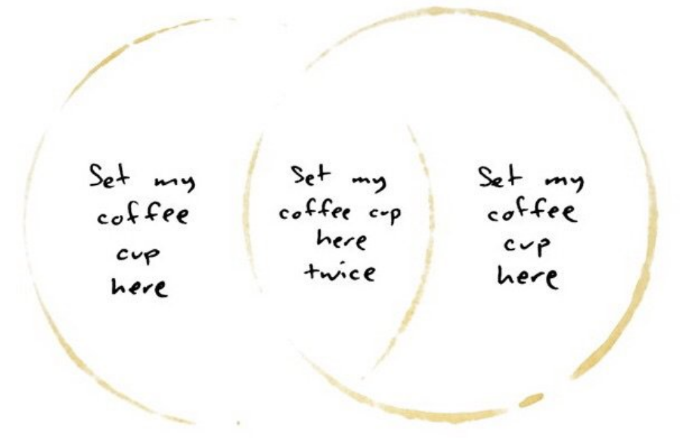


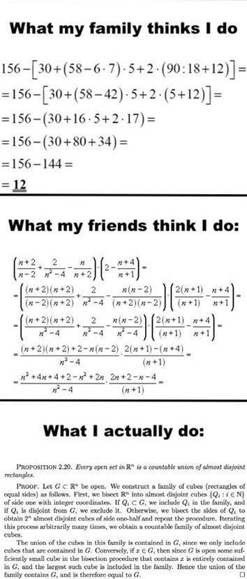
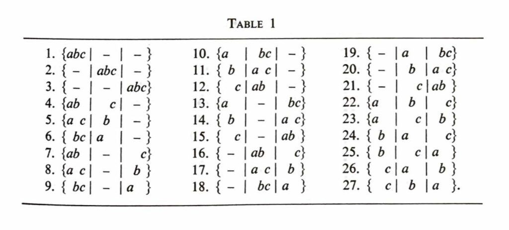
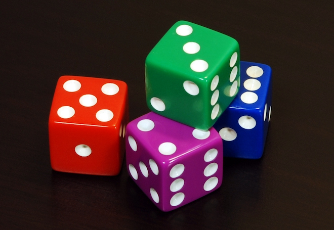
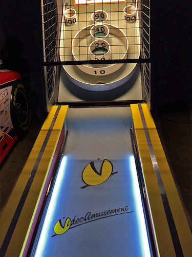
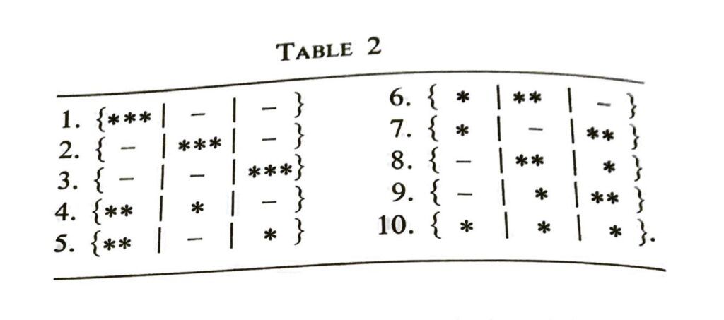


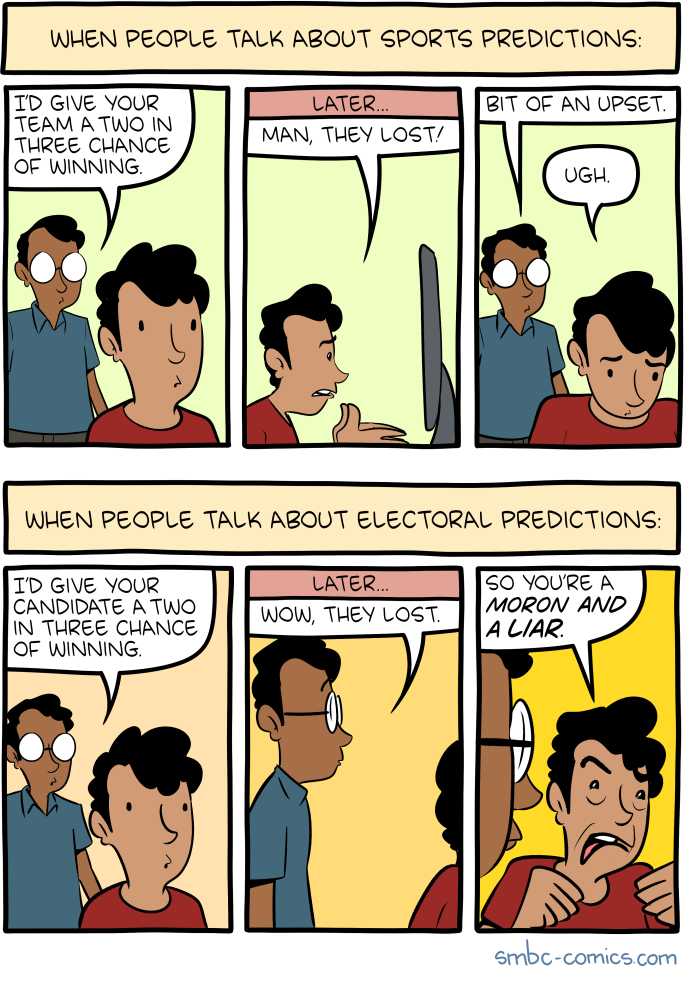
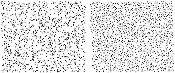
![[Comic: teacher talking to students]
"OK young beings, this is the schedule for this revolution's knowledge transmission"
"This is how I will impart knowledge and prepare you for existence."
"Will we follow this schedule precisely and complete it?"
"Not at all"
"That is how I'll prepare you for existence."
"OK"](https://mcintyre.bennington.edu/wp-content/uploads/2020/08/sp-syllabus-1.png)


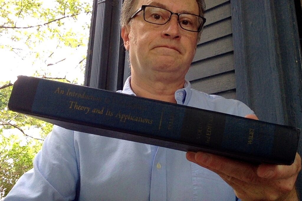
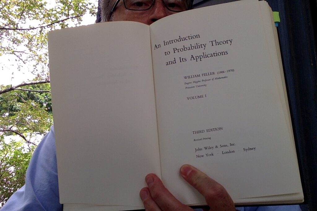

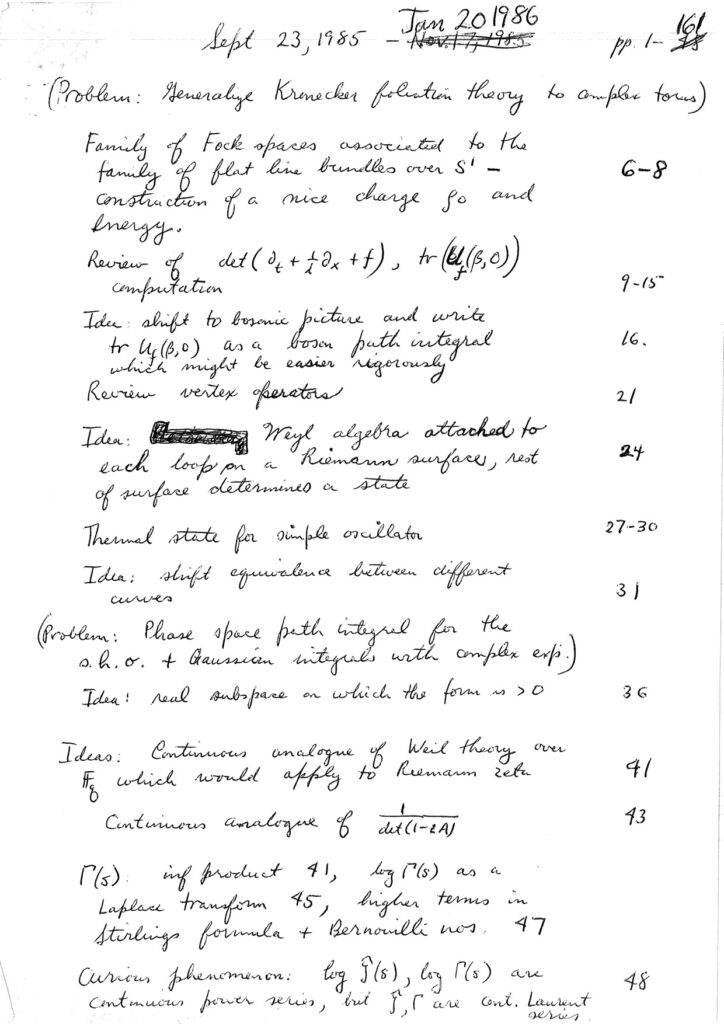
![Comic with parent and child.
Parent: "What is causing distress"
Child: "I just wish to be a grown being so I can commit errors without my instructor marking them"
Parent: "This is unpleasant. And it is true I commit errors and no being marks them. Then other beings who need my precision commit errors and the cumulative consequences of my error expand beyond comprehension"
Parent: "It is terrifying to escape scrutiny"
[Parent stares into space]](https://mcintyre.bennington.edu/wp-content/uploads/2020/09/nathan-pyle-scrutiny-1.png)


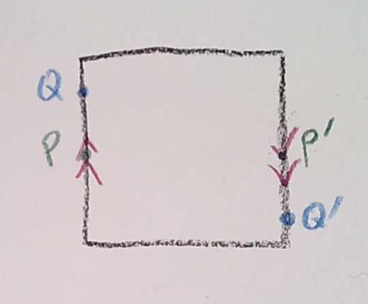
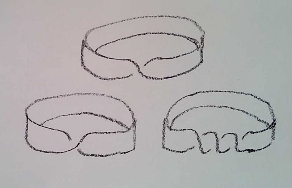
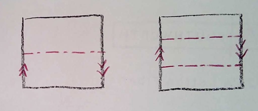
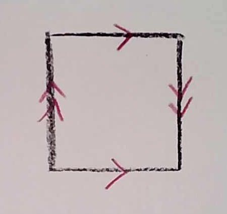
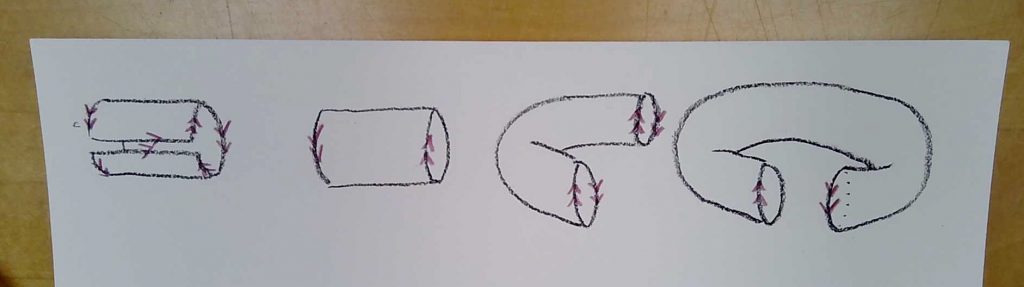

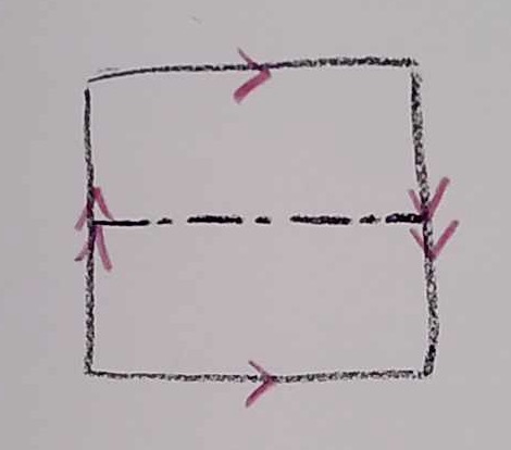
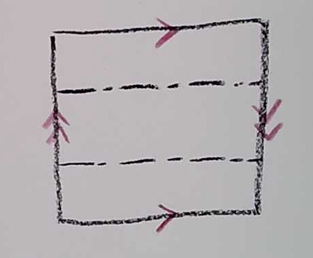


 .
.